Automating GIS Workflows with QGIS (Full Workshop)
A deep dive into the Processing Toolbox for building fast, automated and reproducible workflows.
Ujaval Gandhi
![]()
Note: This workshop is no longer being maintained. You can check out our Advanced QGIS course which covers the same topics in much more depth.
Introduction
This workshop focuses on techniques for automation of GIS workflows and covers the Processing Toolbox in detail. Below are the topics covered in this workshop
- Processing Providers
- Processing Algorithms,
- Processing Modeler
- Batch processing
Get the Data Package
The code examples in this workshop use a variety of datasets. All the
required layers, project files etc. are supplied to you in the zip file
automating_gis_workflows.zip. Unzip this file to the
Downloads directory.
Download automating_gis_workflows.zip
The Processing Framework
QGIS 2.0 introduced a new concept called Processing Framework. Previously known as Sextante, the Processing Framework provides an environment within QGIS to run native and third-party algorithms for processing data. It is now the recommended way to run any type of data processing and analysis within QGIS - including tasks such as selecting features, altering attributes, saving layers etc. - that can be accomplished by other means. But leveraging the processing framework allows you to be more productive, fast, and less error prone.
The Processing Framework consists of the following distinct elements that work together.
- Processing Toolbox: Contains individual tools (i.e. algorithms) grouped by providers and functionality
- Batch Processing Interface: Allows any processing tool to be executed on multiple layers together.
- Graphical Modeler: Allows the user to define the workflow and chain multiple processing steps together using a drag-and-drop mechanism.
- History Manager: Records and stores all executions of algorithms to allow users to reproduce past analysis.
- Results Viewer: An interface to view non-spatial outputs from algorithms - such as tables and charts.
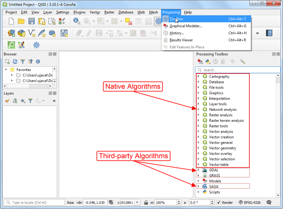
Processing Toolbox
Processing Toolbox is available from the top-level menu Processing → Toolbox. There are hundreds of algorithms available out of the box. They are organized by Providers. The tools created by QGIS developers is available as a Native QGIS provider. Processing Framework providers an easy way to integrate tools written by other software and libraries such as GDAL, GRASS and SAGA. QGIS Plugins can also add new functionality via processing algorithms in the toolbox.
Why should you use Processing Algorithms
- Well tested and rigorous implementations
- Majority are written in C++ and are faster than alternatives
- Long processes can run the the background while you continue to use QGIS
- Many multi-threaded algorithms can take advantage of multi-core CPU on your machines and give you better performance
- Robust handling of invalid geometry
- Ability to see progress of the operation and cancel it
- Easily run on all or just selected features
Exercise: Find the length of interstate highways in each state of the US
The aim of this exercise is to show how a multi-step spatial analysis problem can be solved using a purely processing-based workflow. This exercise also shows the richness of available algorithms in QGIS that are able to do sophisticated operations that previously needed plugins or were more complex.
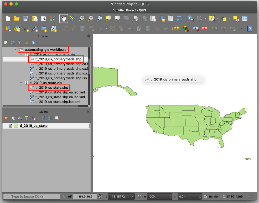
We will work with shapefiles provided by US Census Bureau. The
tl_2019_us_primaryroads.zip file comes TIGER/Line roads
database and contains all the major roads in the US - including
Interstate highways. The tl_2019_us_state.zip file comes
from the Cartographic Boundary Files and contains the state
boundaries.
- Browse to the data directory and expand
tl_2019_us_primaryroads.zipandtl_2019_us_state.zipfiles. Drag and drop thetl_2019_us_primaryroads.shpandtl_2019_us_state.shplayers to the canvas.
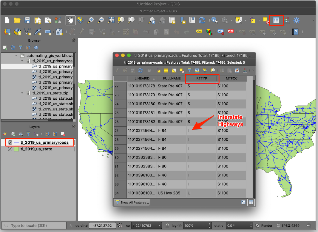
- The layer
tl_2019_us_primaryroadscontain all major roads, including interstate highways, state highways, US highways etc. Select the layer and use the keyboard shortcut F6 to open the attribute table. You will notice that theRTTYPcolumn has information about road designation. As we are interested in only interstate highways, we can use the information in this column to extract relevant road segments.
Note: The roads layer has 2 line segments per road, representing the route in both directions.
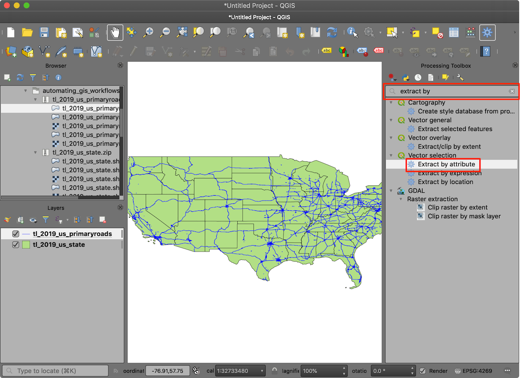
- Open the Processing Toolbox by going to Processing → Toolbox
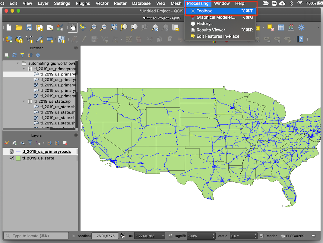
- You can use tools such as Select by expression, export the selected features as a new layer and continue to work. But the processing toolbox providers a better and seamless workflow. Search for the algorithm Extract by attribute.
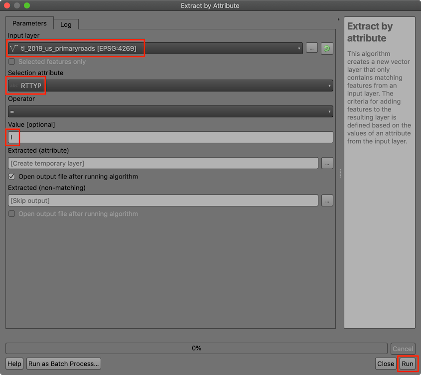
- Select
tl_2019_us_primaryroadsas the Input layer. SelectRTTYPas the Selection attribute andIas the Value. This will extract all feature where RTTYP value is I (Interstate). Click Run.
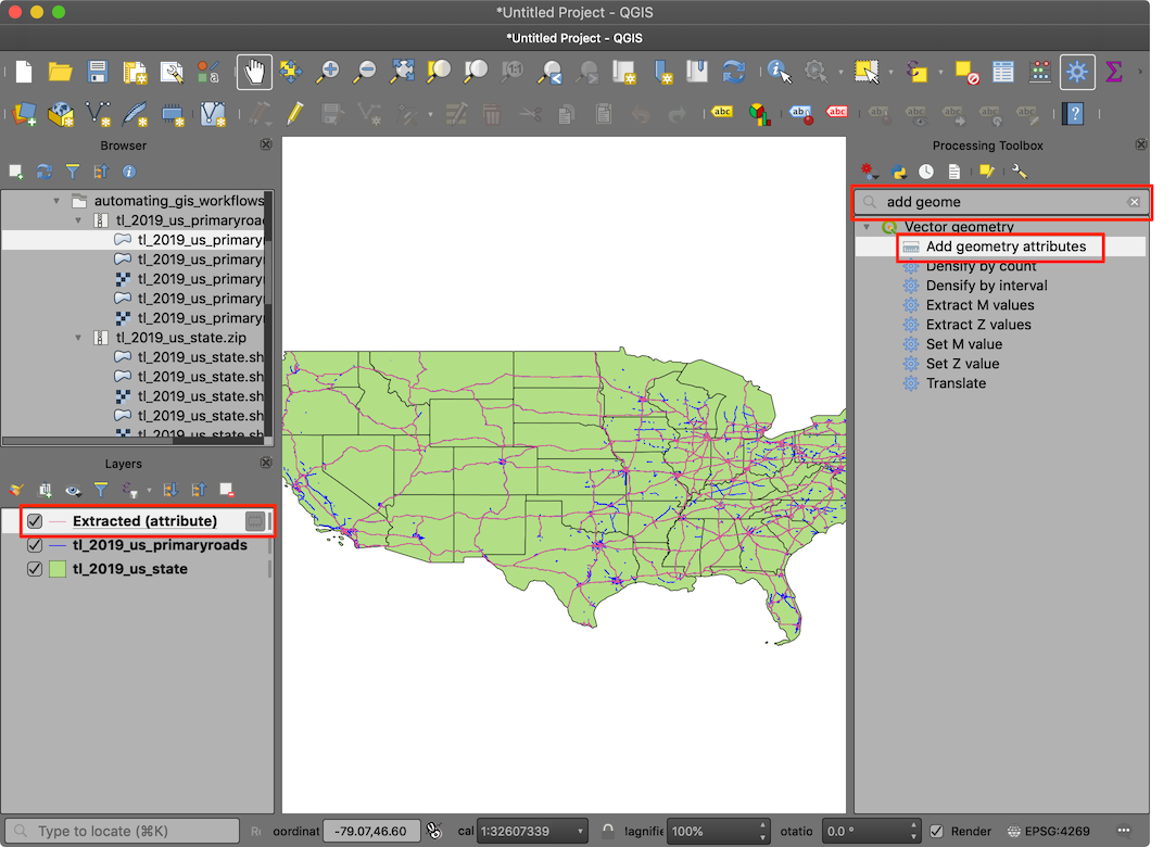
- You will get a new layer
Extracted (attribute)in the Layers Panel. Next, we want to calculate the length of each segment. You can use the built-in algorithm Add geometry attributes
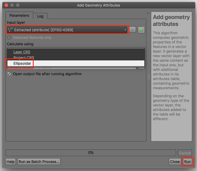
- The source layer is in the Geographic CRS EPSG:4269 (NAD83) with
degrees as units. But for the analysis, we want the lengths to be
measured in linear units - such as miles. The algorithm provides us with
a handy option to calculate the distances in
Elliposidal math - which is ideal for layers in the
geographic CRS. Select
Extracted (attribute)as the Input layer, selectEllipsoidalas Calculate using and click Run.
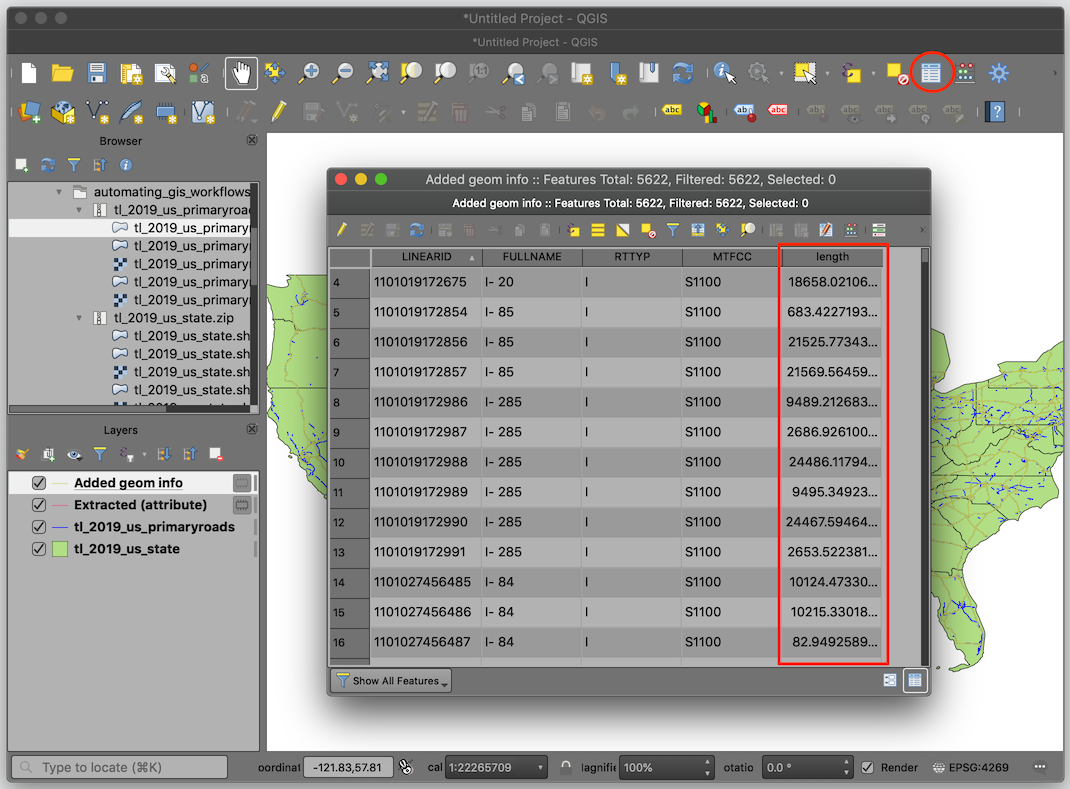
- A new layer with an additional field called
lengthwill be added to the Layers panel. The distances in this field are in meters.
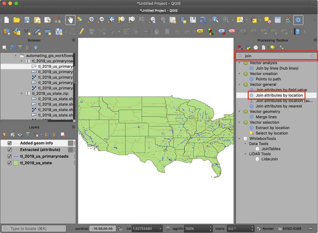
- We have the state information in the
tl_2019_us_statelayer, but not in the roads layer. To add the name of the state to the roads layer, we need to perform a spatial-join. This is done using the Join attributes by Location algorithm.
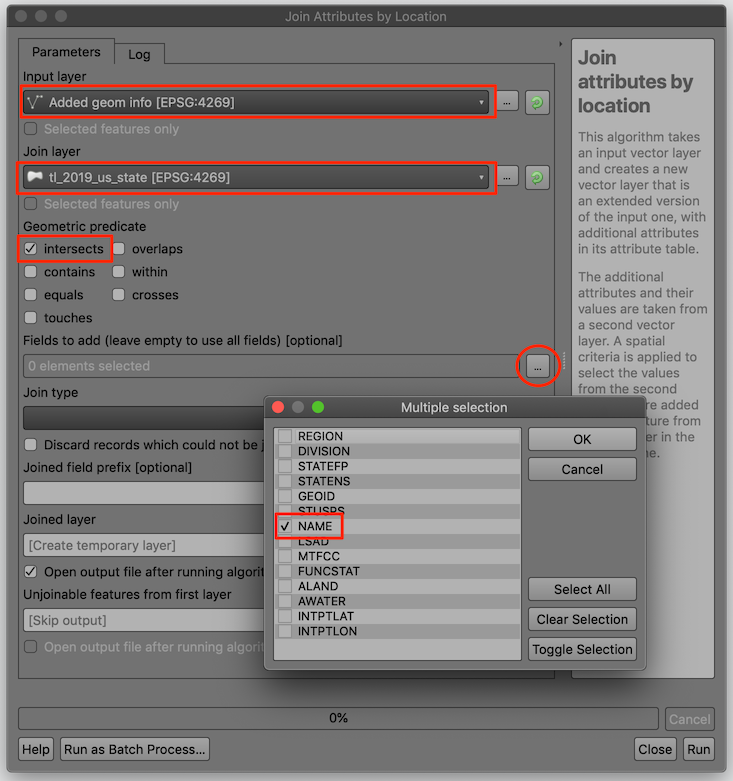
- Select the
Added geom infoas the Input layer andtl_2019_us_stateas the Join layer. For the Fields to add, we need only theNAMEof the state.
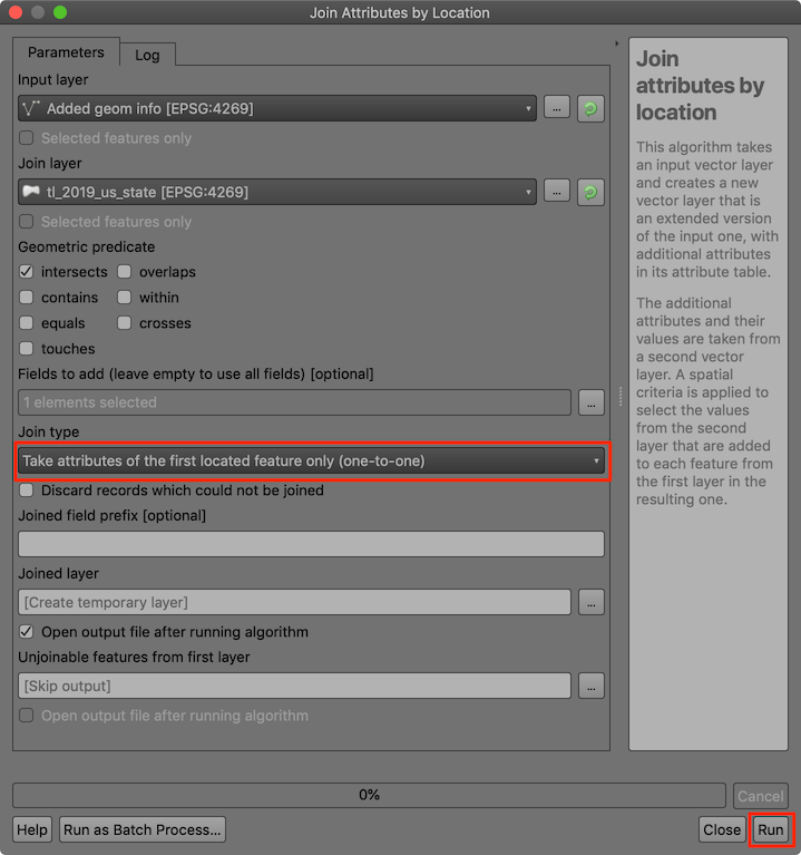
- Fortunately for us, each road segment is split at the state
boundary. So we can select
Take attribute of the first located feature onlyand click Run to perform a one-to-one join.
If our input road layers had segments that crossed state lines, we would have to do an extra step of splitting them so when we count road lengths per state - we get accurate results. You may do this by converting the states layer to lines using Polygons to lines algorithm, followed by the Split by Lines to split the road segments at the boundary.
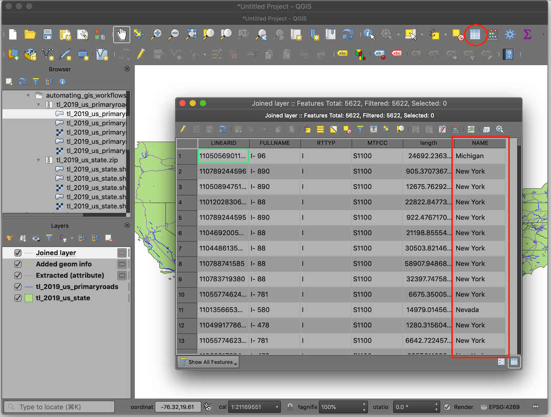
- The new layer
Joined layernow has the state name for every road segment.
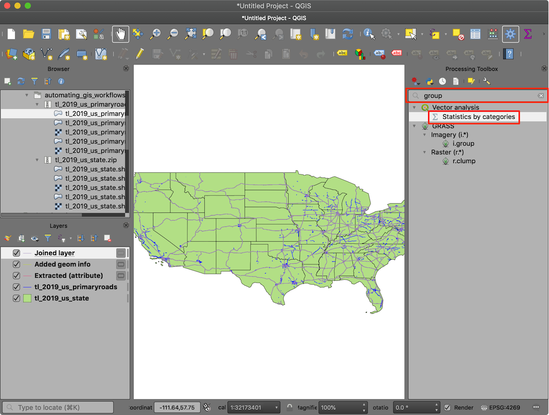
- We can now sum the road lengths and group them for each state You may recall that in earlier versions of QGIS, you needed a plugin called Group Stats to do this. But now we can do this via the built-in Statistic by Categories algorithm.
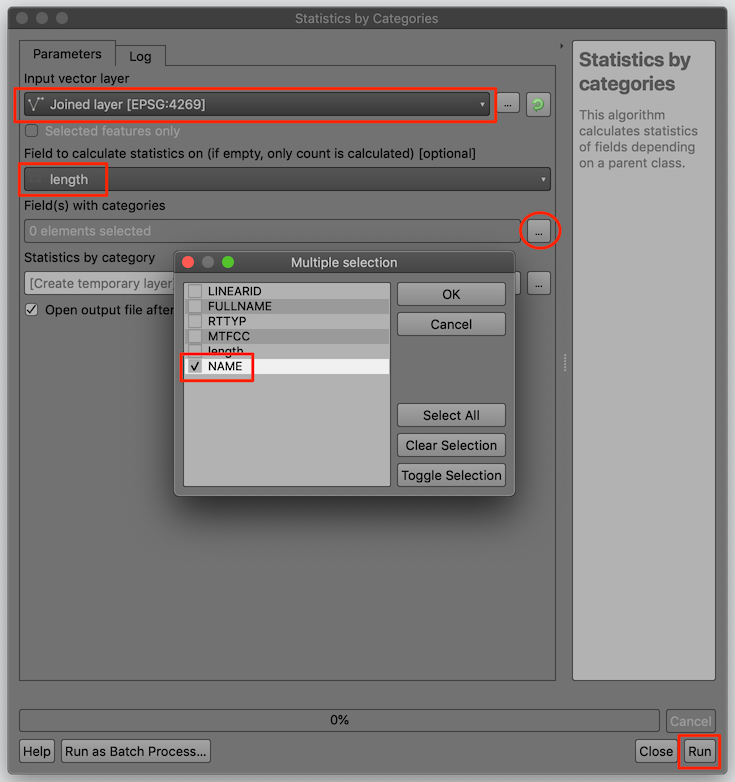
- Select
Joined layeras the Input vector layer. We want to calculate lengths, but group them by states. So selectlengthas the Field to calculate statistics on andNAMEas the Field(s) with categories. Click Run.
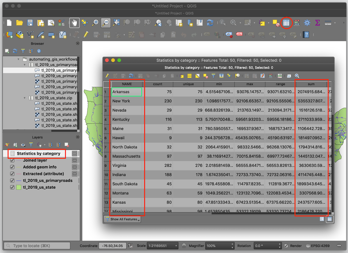
- The output of the algorithm is a table containing various statistics
on the
lengthcolumn for each state. The values in the sum column is the total length of national highways in the district.
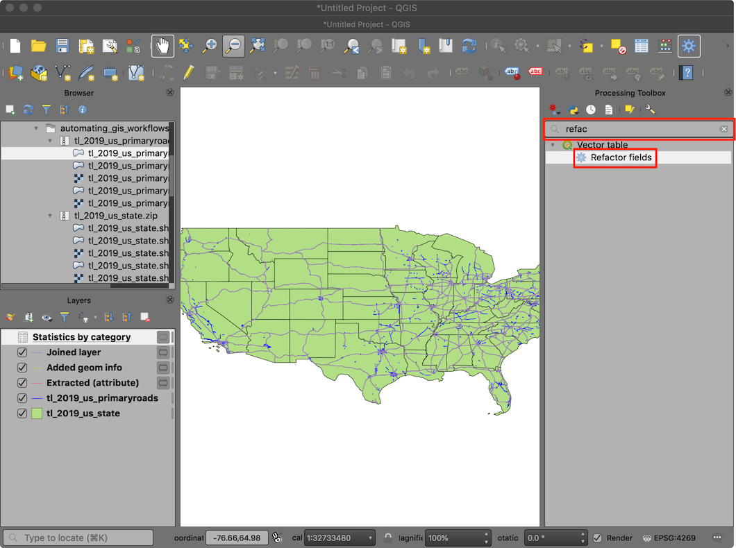
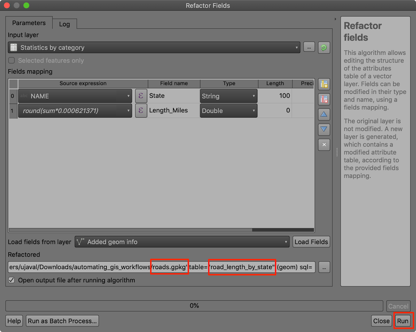
- The layer contains many fields which are not relevant to us, so let’s delete some columns before saving. The classic way to do this is to toggle editing and use the Delete Column button from the Attribute Table. If you wanted to rename/reorder certain fields, that needed a plugin. But now, we have a really easy processing algorithm called Refactor Fields that can add, delete, rename, re-order, re-calculate and change the field types all at once.
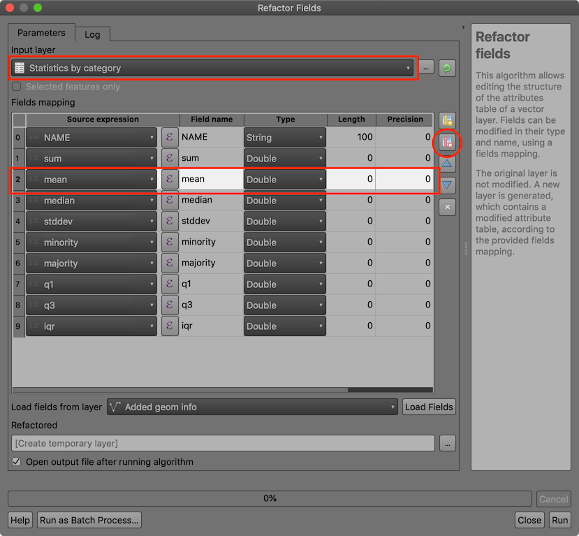
- In the Refactor fields dialog, select rows containing
fields that you want to delete and click the Delete selected
field button. Delete all except the
NAMEandsumfields.
- The lengths contained in the
sumfield is in meters. We can convert it to miles here itself. Click the button next tosumin the Source experssion column and enter the following expression that converts meters to miles and rounds the value to the nearest integer. Click OK.
round(sum*0.000621371)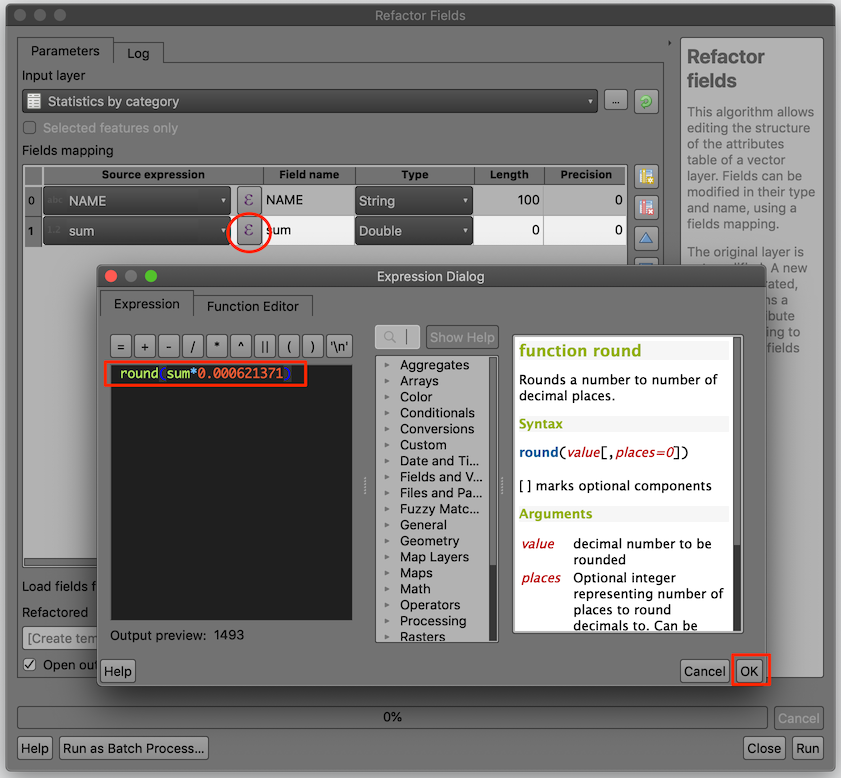
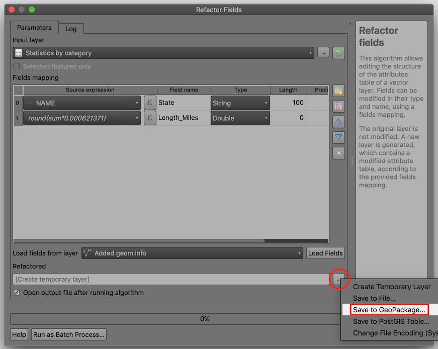
- We can also rename the field to a better name. Change the Field
name of
NAMEtoStateandsumtoLength_Miles. We are ready to apply the changes. So far we have created temporary output layers, but this is the final result of the analysis, so we can save it to the disk. Click the...button at the bottom and selectSave to GeoPackage.
- Enter the name of the file as
roads.gpkg. When prompted for a layer name, enterroad_length_by_state. Click Run.
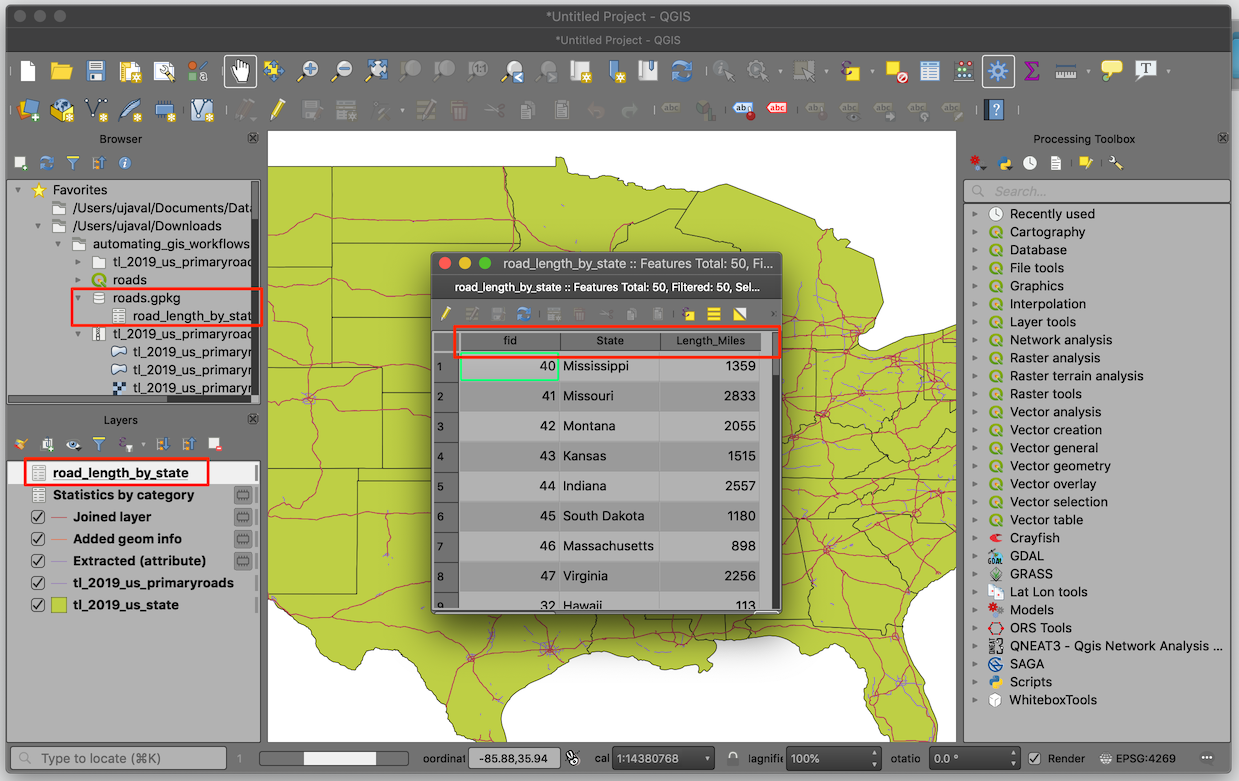
- A new layer
road_length_by_statewill be added to the Layers panel. The table will have the fields renamed and re-calculated as we had specified.
Note: The refactor fields algorithm has a bug for the Mac version that makes all fields as strings regardless of the user’s choice. This is a known issue and will be fixed in the future version. Till then, if you are on Mac, a workaround is to use the Field Calculator algorithm to take the result and add fields with correct types and conversion expressions such as to_int(), to_double() etc.
Note that we did data processing, spatial analysis and statistical analysis - all using just processing algorithms in a fast, re-producible and intuitive workflow.
Lesser Known Algorithms
The Processing Toolbox contains hundreds of algorithms - with new ones being added everyday. Many plugins also add processing algorithms that support new functionality. While you may think that processing algorithms are meant for analysis - there are plenty of algorithms that offer functionality that is beyond geoprocessing. Here are a few algorithms that I find very useful to automate my workflows that you may not be aware of.
Download file: Download file from a URL or FTP site. Allows you to automate tasks where you need to download new data regularly and process it.Import geotagged photos: Extracts latitude, longitude and azimuth information from a directory of photos and creates a point layer.Add autoincremental field: Simple but very useful algorithm to add a unique integer field. Many databases (even geopackage) requires that each layer has a unique integer field. This algorithm helps creating this field if your source layer doesn’t have one. CAD or CSV layers frequently have this problem.Create spatial index: Spatial indexes speed up your geoprocessing operation a lot. This algorithm can create spatial indices on many types of layers, including those loaded from a database.ORS Tools Algorithms: OpenRouteService (ORS) provides a QGIS plugin which installs a slew of network analysis algorithms to the Processing Toolbox. They allow rich network analysis functionality using OpenStreetMap data and it works without having to download any data.
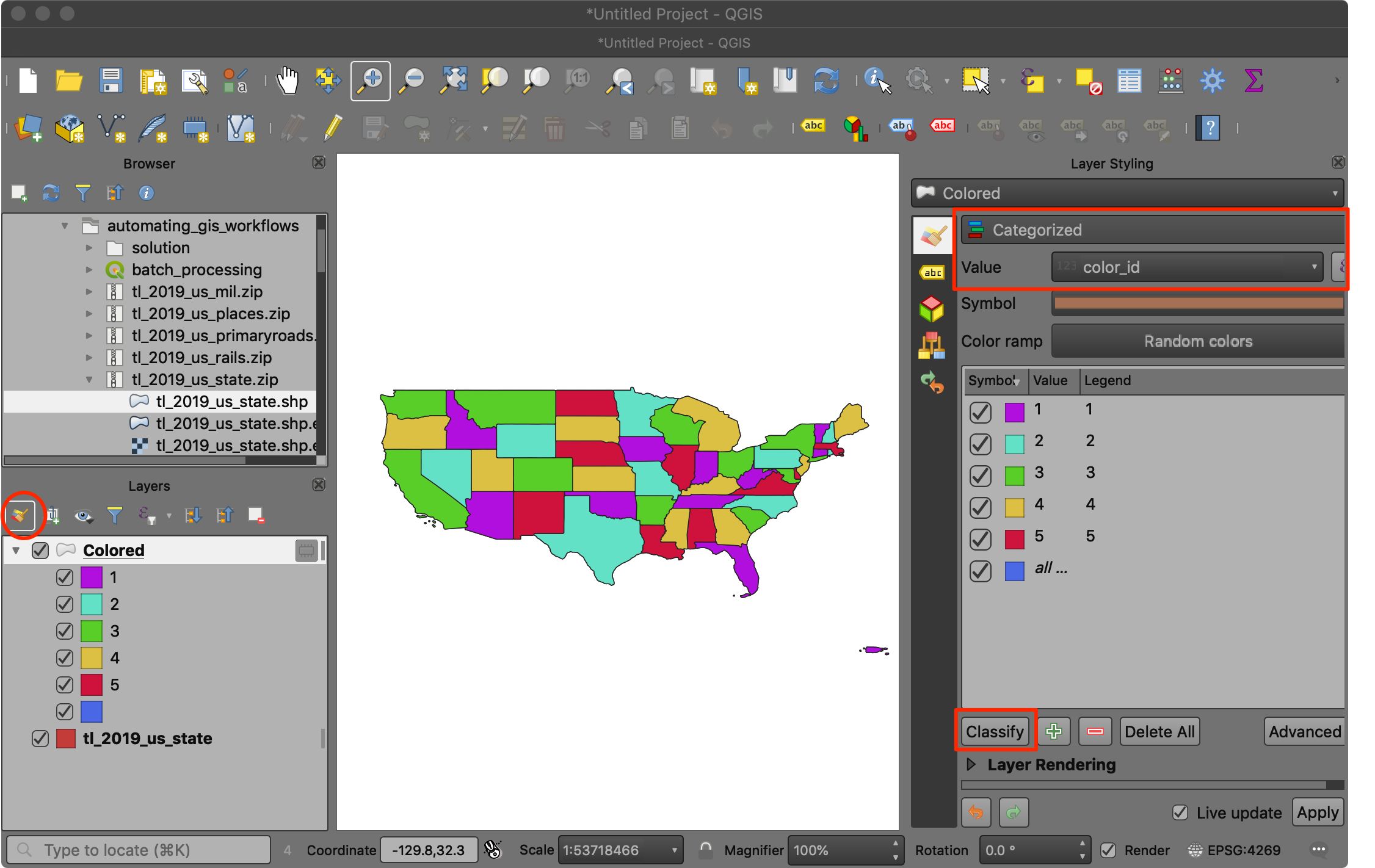
A fun and interesting algorithm is called
Topological coloring. This algorithm implements helps with cartography by allowing you assign a color_id to your polygon layers such that no adjacent polygons have the same color.
Graphical Modeler
As we saw in the previous example, GIS Workflows typically involve many steps - with each step generating intermediate output that is used by the next step. If you change the input data or want to tweak a parameter, you will need to run through the entire process again manually. Fortunately, Processing Framework provides a graphical modeler that can help you define your workflow and run it with a single invocation. You can also run these workflows as a batch over a large number of inputs.
Exercise: Build a model to calculate road lengths
We will take the workflow from the previous section and build a model that can precisely reproduce all the intermediate steps and give us the result. The model will allow us to specify the input layers and parameters and perform all intermediate steps without any user input. This will greatly speed up our analysis and ensure we do not make manual errors when running the same calculations again.
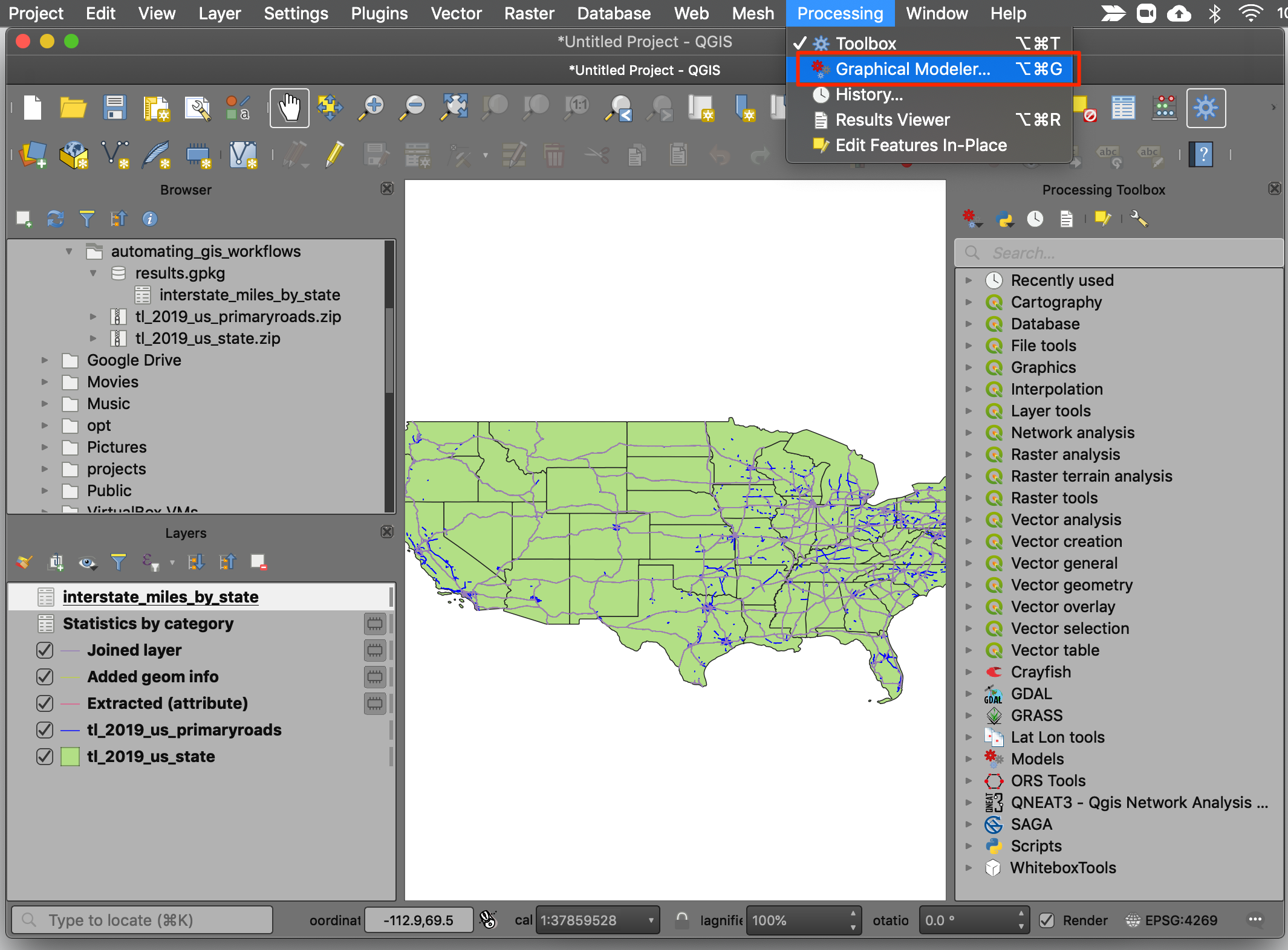
- Open the modeler tool from Processing → Graphical Modeler.
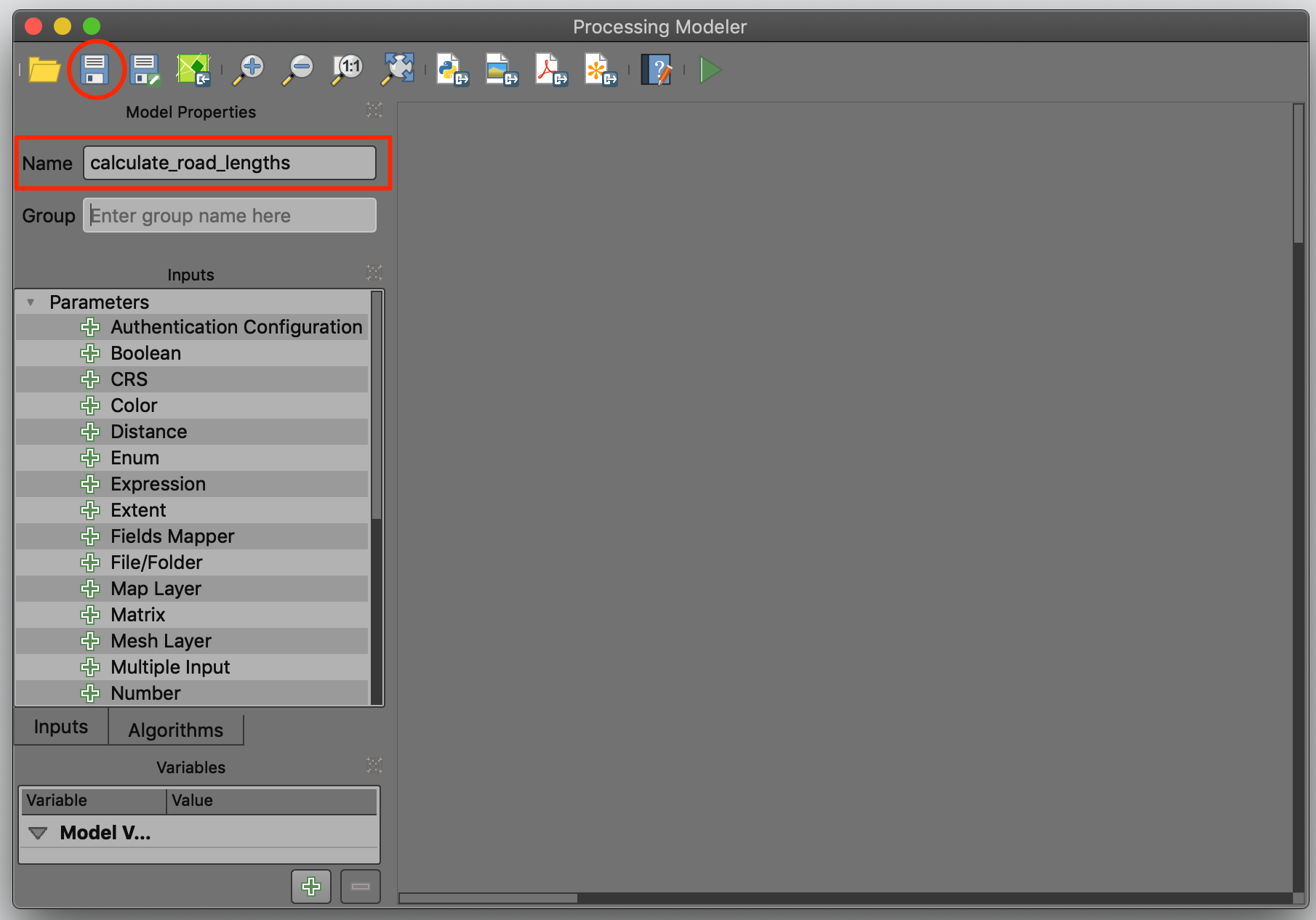
- Enter the name of the model as
calculate_road_lengthsand click the Save button. Save the model ascalculate_road_lengths.model3file at the default location.
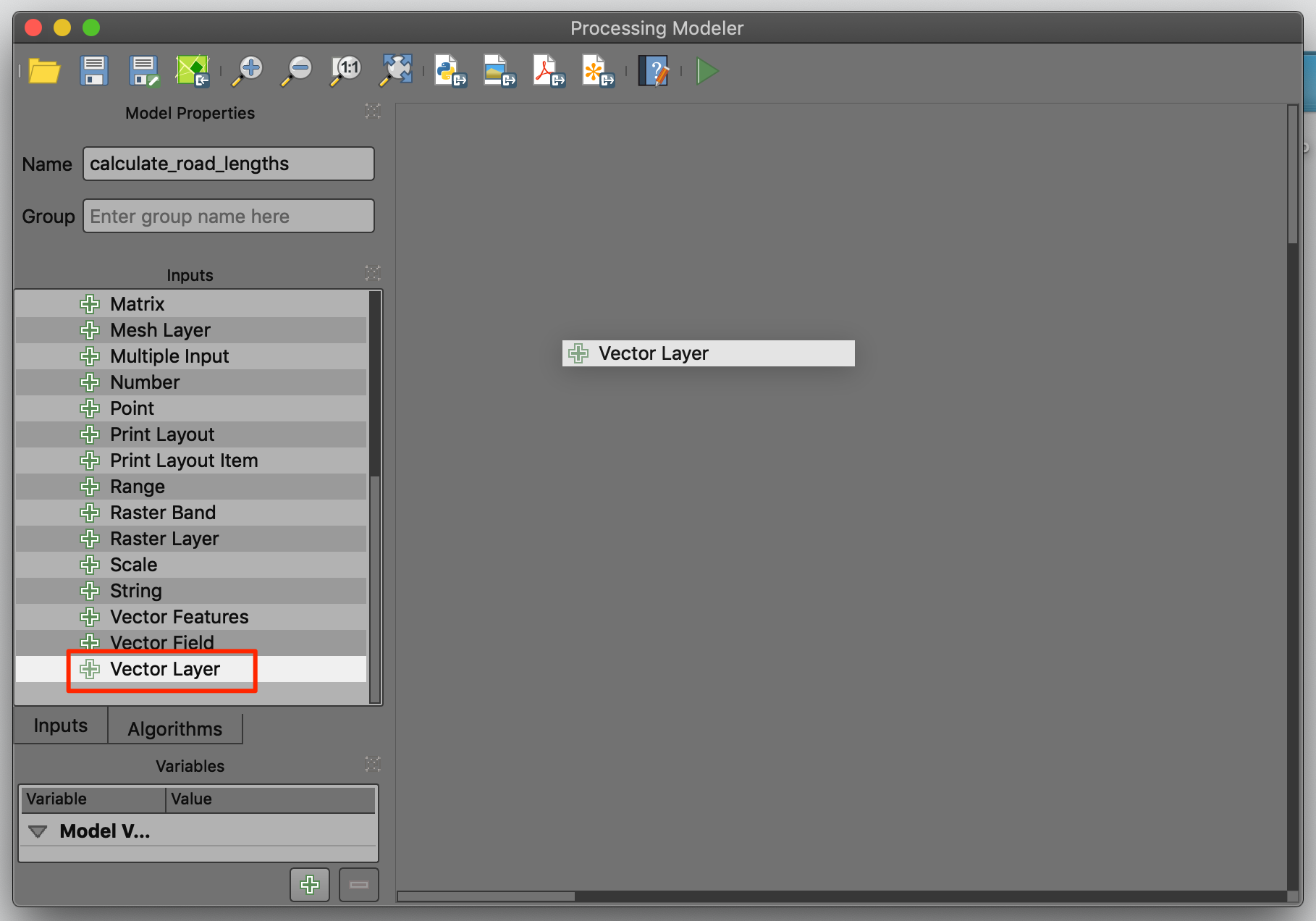
- The modeler interface contains the left-hand panel with 2 tabs -
Inputs and Algorithms. Our first step is to define the
inputs to the model. In our case, the inputs are the 2 vector layers -
primary roads and states. Find the
Vector Layerinput and drag it to the canvas.
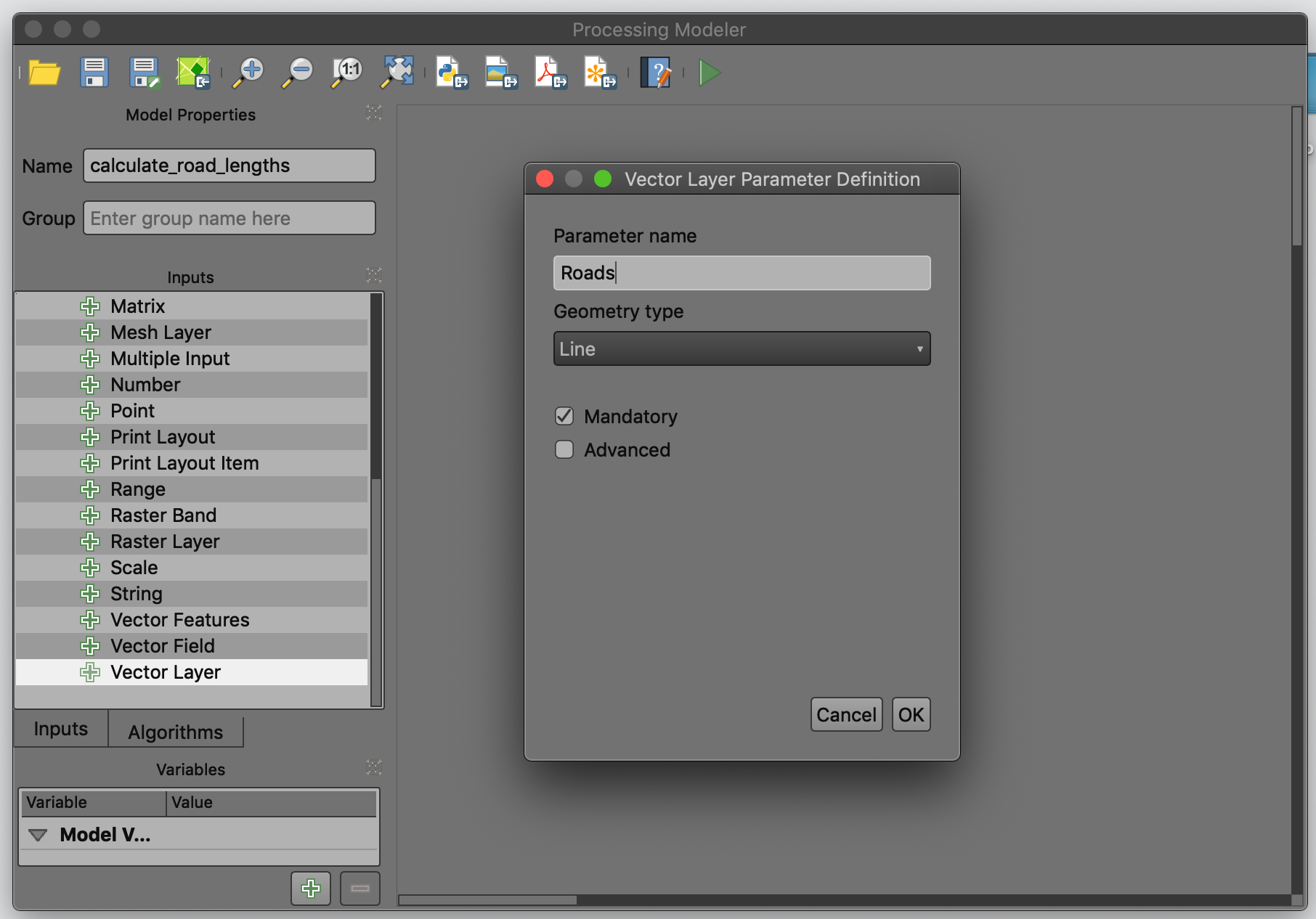
- In the Vector Layer Parameter Definition dialog, enter
Roadsas the Parameter name and setLineas the Geometry Type. Click OK.
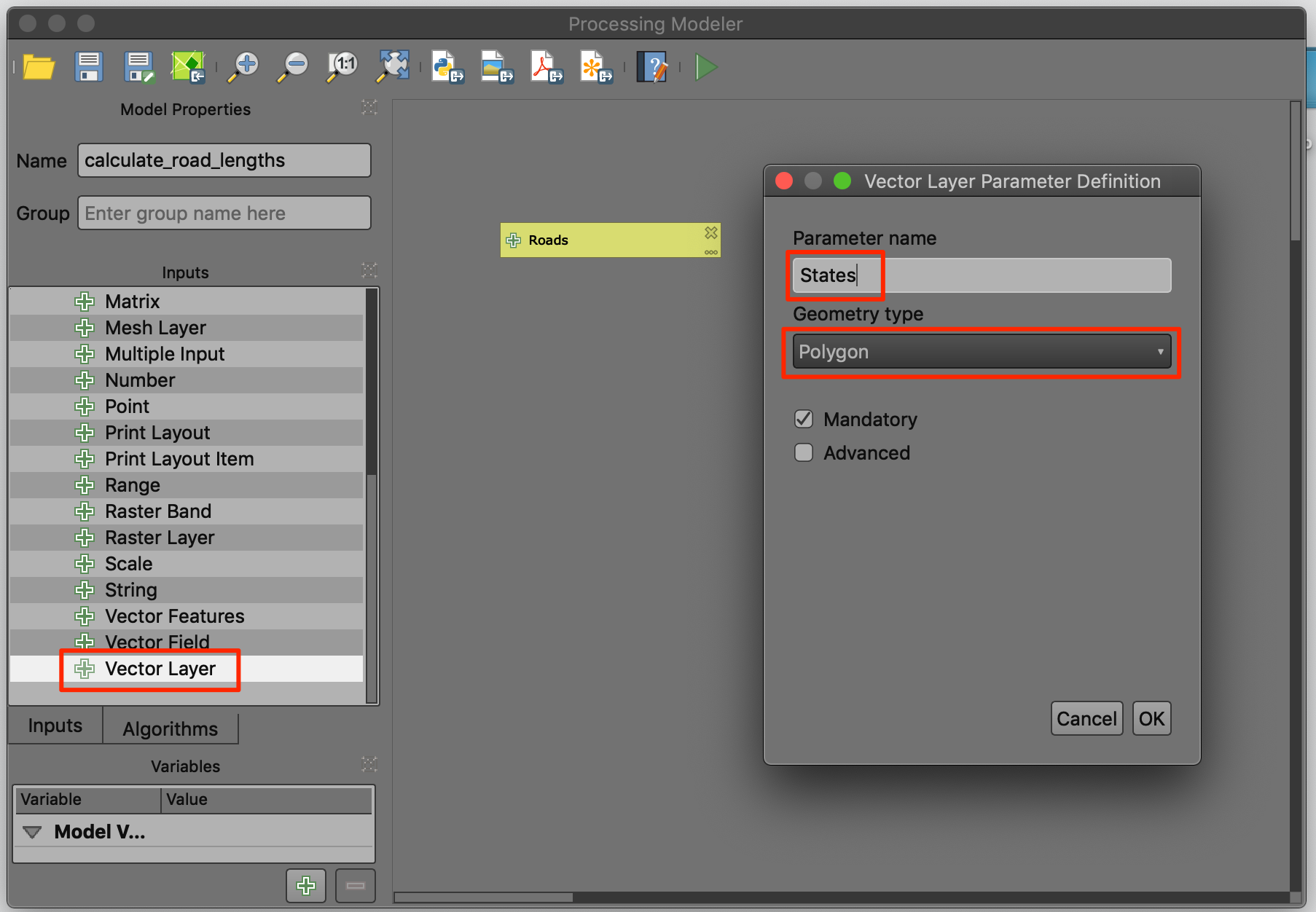
- Similarly, drag another
Vector Layerinput.Statesas the Parameter name and setPolygonas the Geometry Type. Click OK.
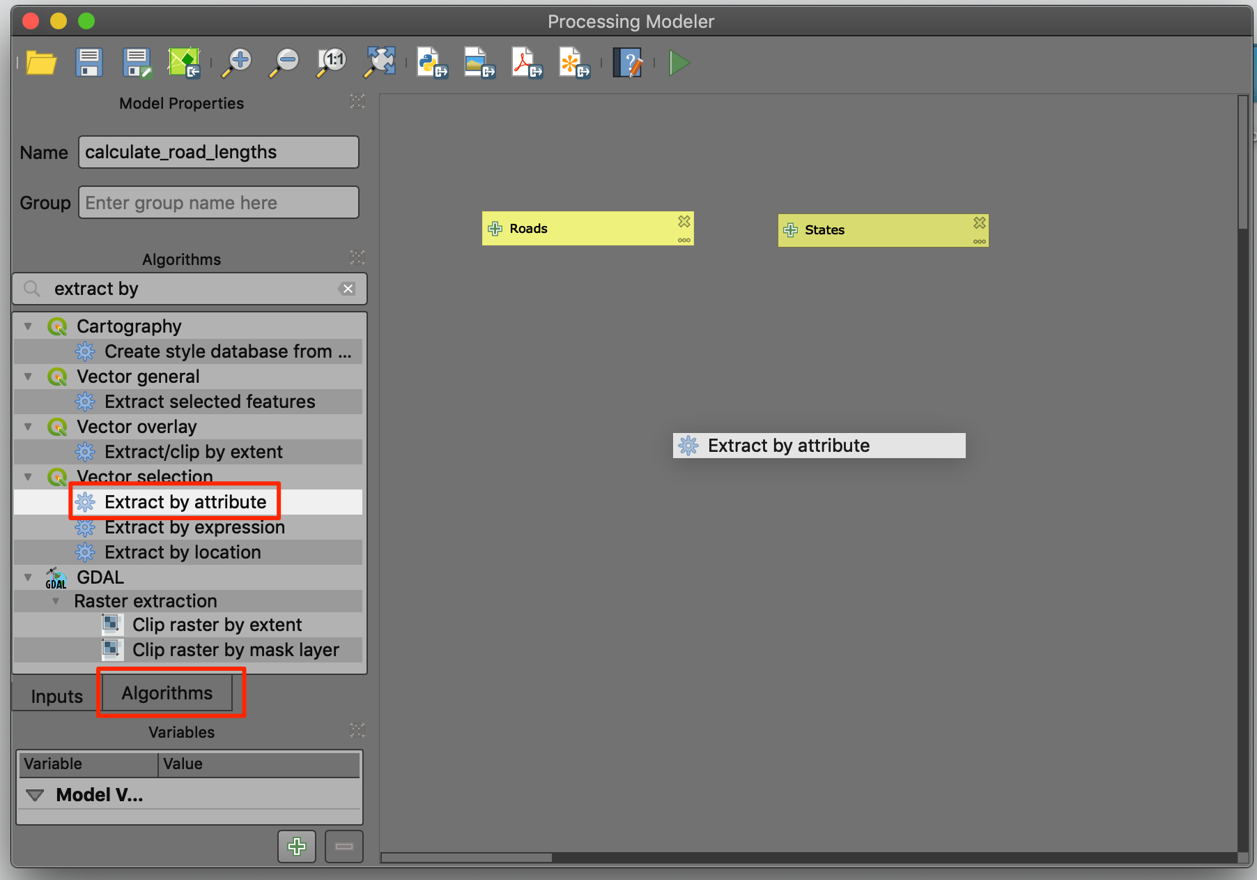
- You should have 2 boxes representing the input layers. Now switch to
the Algorithms tab and search for the
Extract by attributealgorithm. Drag it to the canvas.
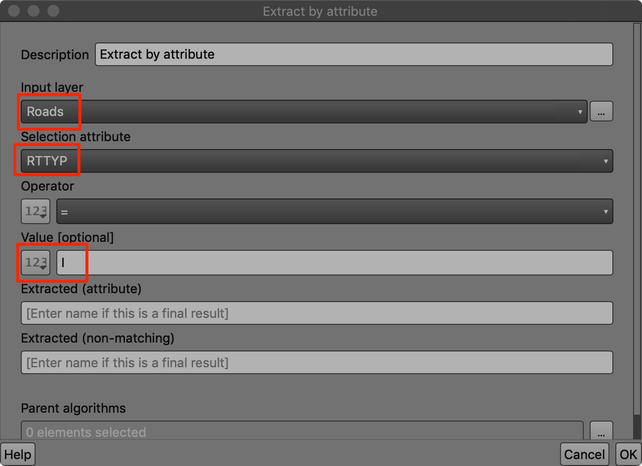
- Fill in the parameters the same way we did in the previous exercise.
Roadsas the Input layer,RTTYPas the Selection attribute andIas the Value. Click OK.
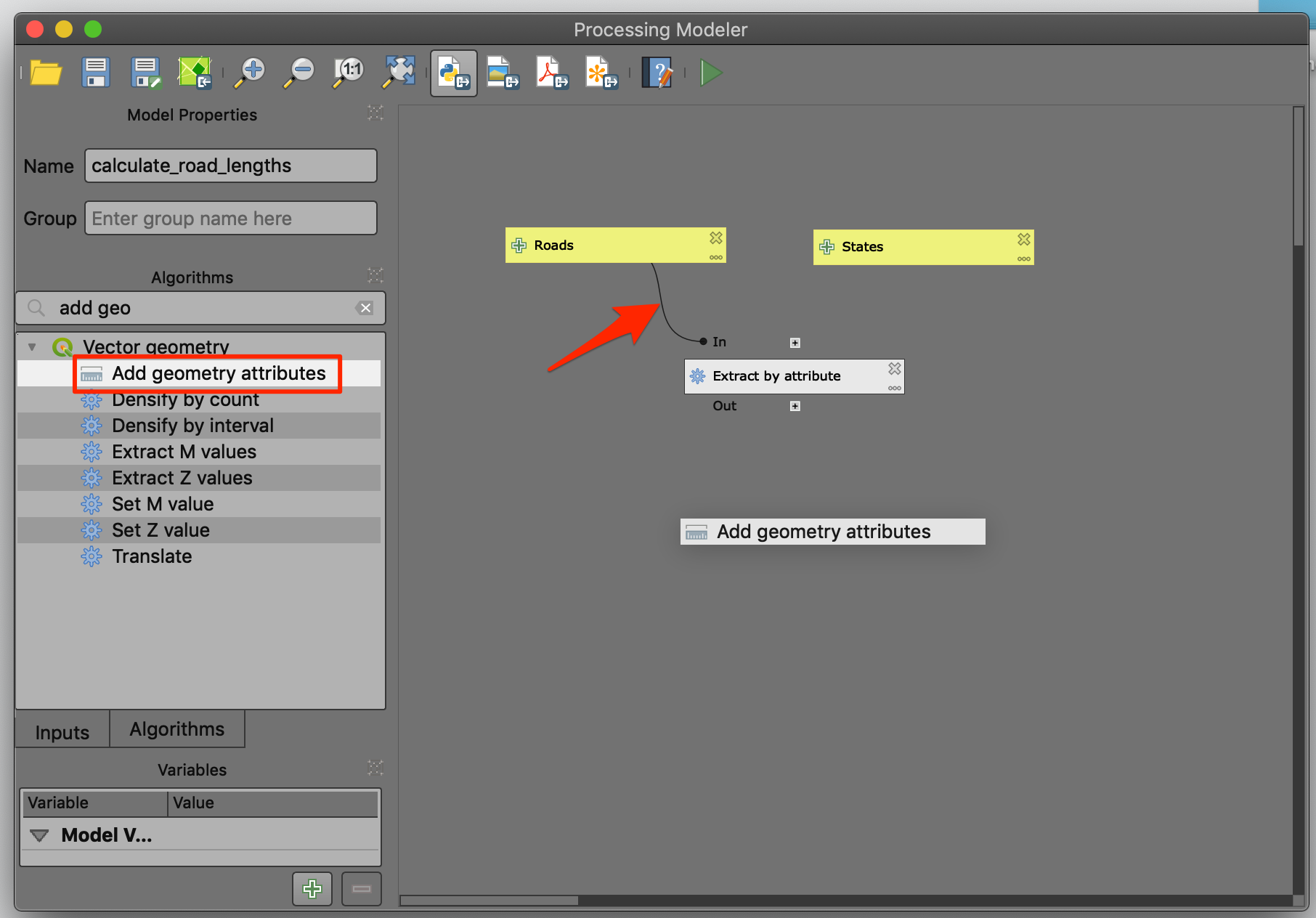
- In the modeler canvas, you will see a new box with the Extract
by attribute algorithm and an arrow connecting it with one of the
inputs. This indicates that the algorithm is using that input for
processing. Next search for and add the
Add geometry attributesalgorithm.
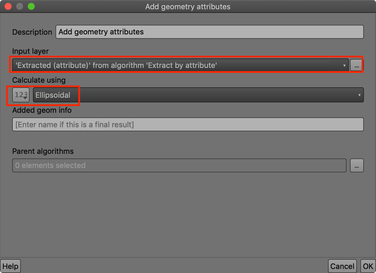
- Set the
'Extracted (attribute)' from algorithm 'Extract by Attribute'as the Input layer. SelectEllipsoidalas the method for Calculate using. Click OK.
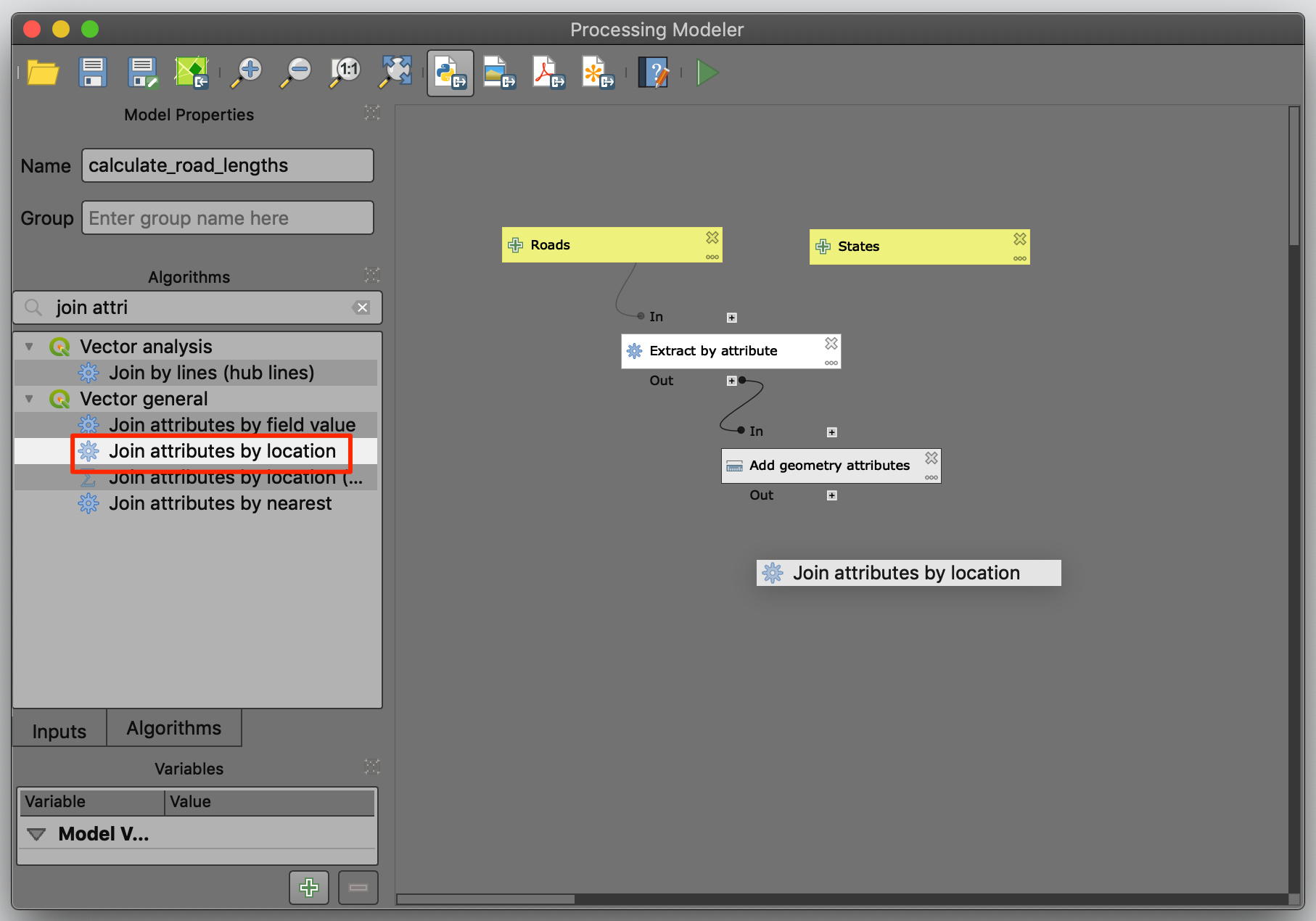
- Referring back to the previous example, the next step in the
processing is doing a spatial join. Search for and add the
Join attribute by locationalgorithm.
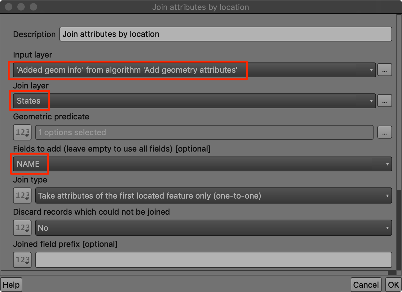
- Set the
'Added geom info' from algorithm 'Add geometry attributes'as the Input layer. The Joim layer will be theStateslayer. In the Fields to add, enterNAME. Click OK.
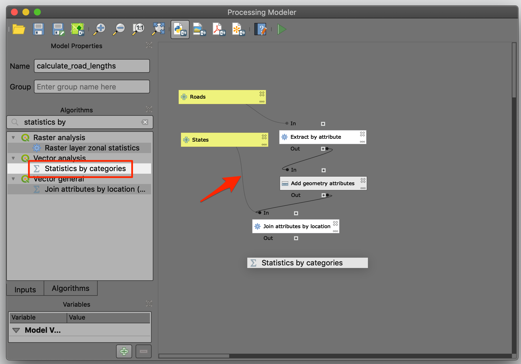
- In the canvas, you will see another arrow now connecting the
Statesinput to theJoin attributes by locationbox. Next, add theStatistics by categoryalgorithm.
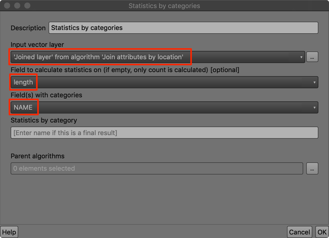
- Set the
'Join layer' from algorithm 'Join attribues by location'as the Input vector layer. Enterlengthas the Field to calculate statistics on andNAMEas the Field(s) with categories. Click OK.
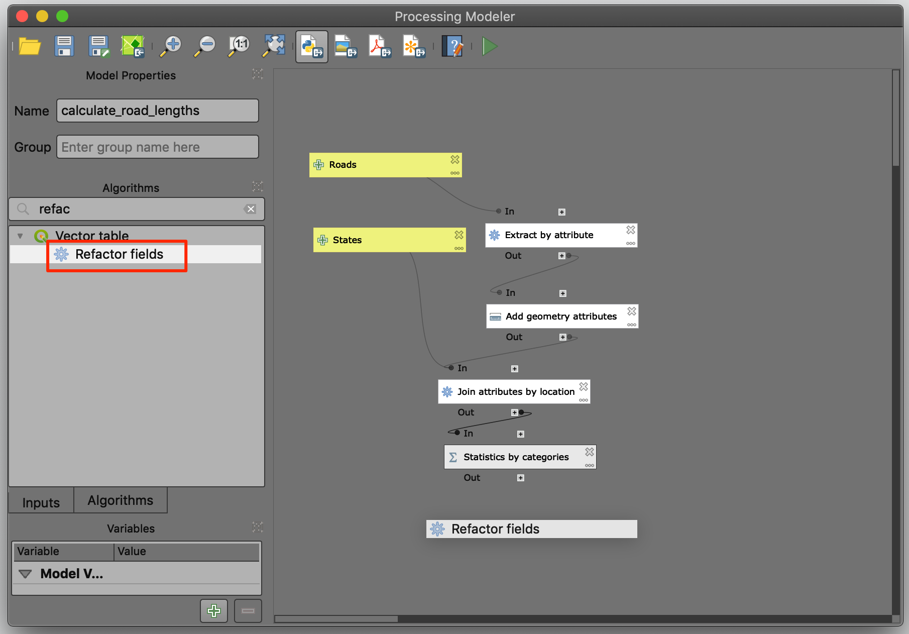
- We are at the last step now. Add the
Refactor fieldsalgorithm.
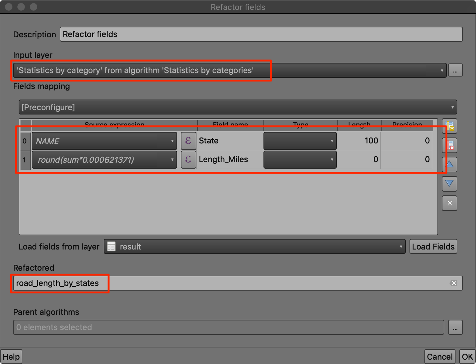
- Set
'Statistics by category' from algorithm 'Statistics by categories'as the Input layer. The Field mapping table is empty. We need to add rows for the fields that we want in the output. Click Add new field twice to add 2 rows. Configure the rows to match our input in Step 19 from the previous exercise. As this is the final result, we should specify the name of the output layer. Enterroad_length_by_statesas Refactored. Click OK.
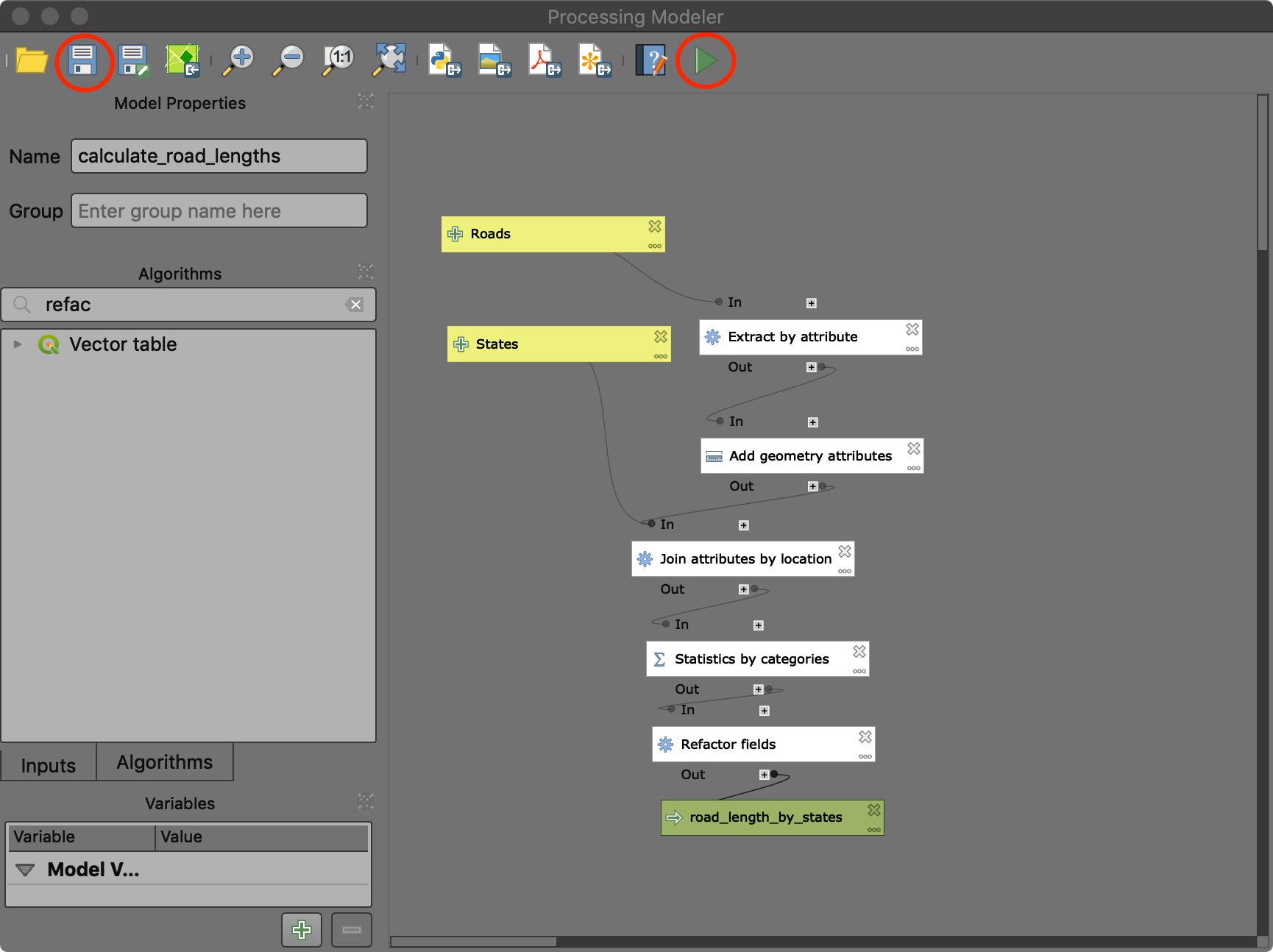
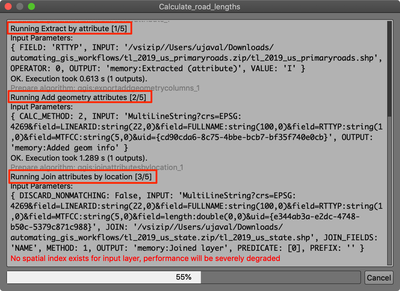
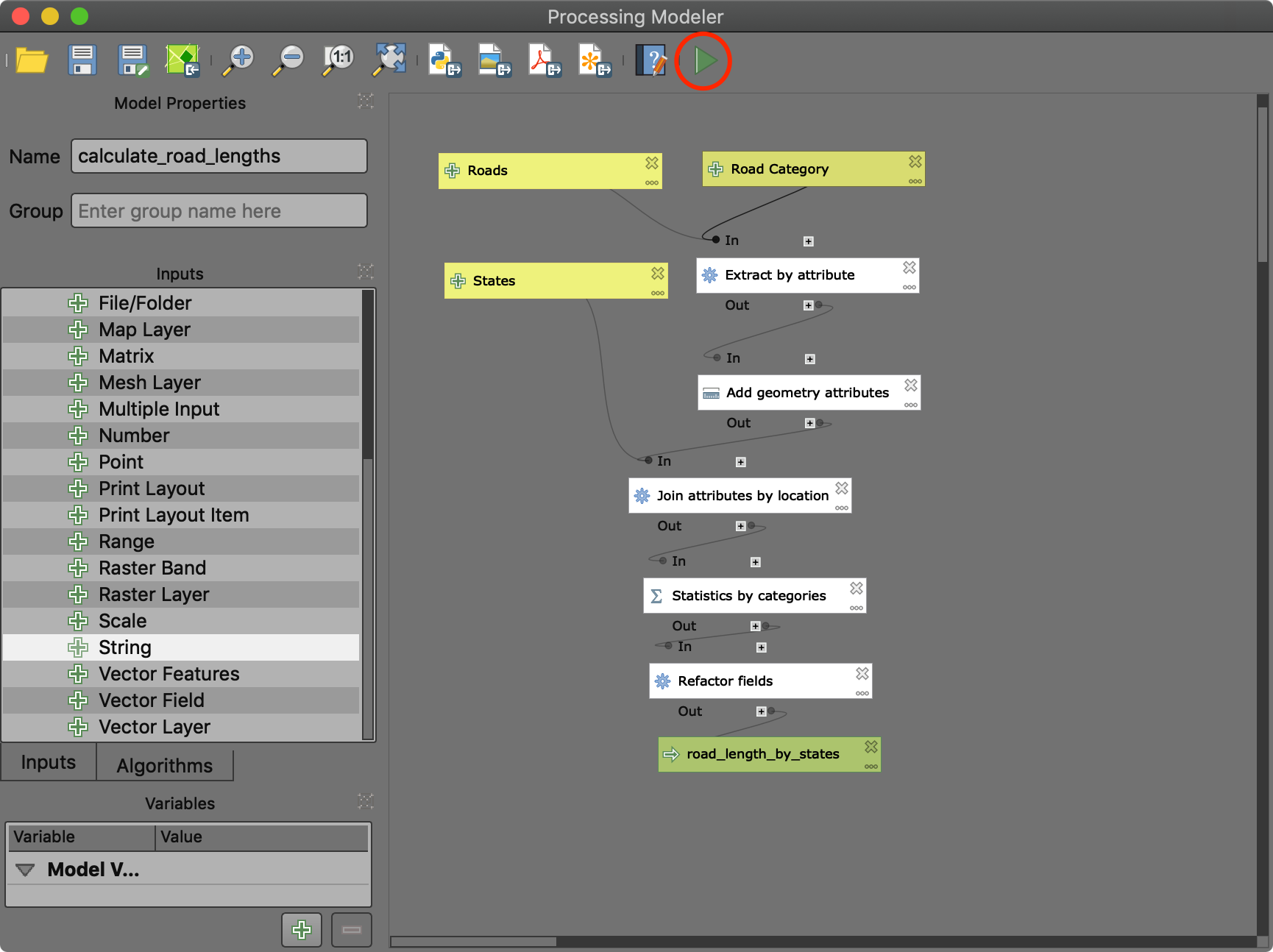
- The model is ready to run. Click the Run button.
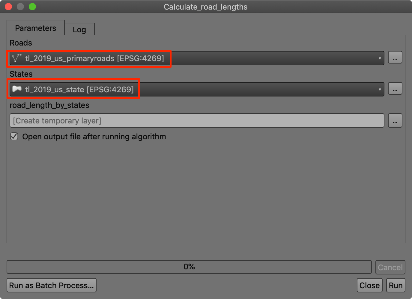
- Set
tl_2019_us_primaryroadsas Roads andtl_2019_us_statesas States. Click Run.
- As the model runs, you will each step of the process being run and intermediate results generated.
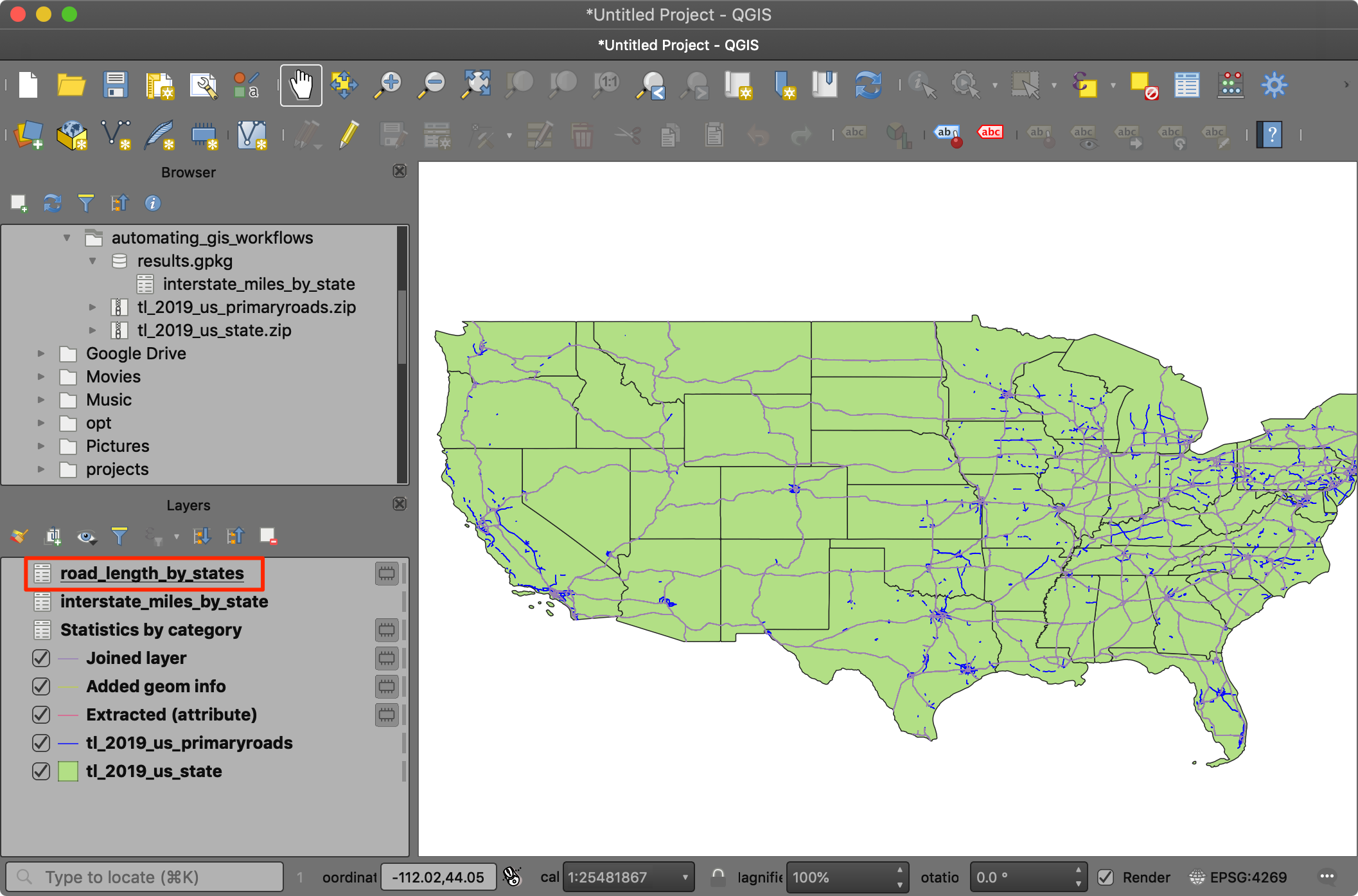
- Once the process finishes, you will see only 1 new layer - our final result, loaded to the Layers panel. You can verify that the result is exactly the same as our manual processing in the previous example. But this time, we only had to specify the inputs and the model did all the hard work.
- Let’s learn how to improve this model. We can generalize this model
a little to calculate lengths of not only interstate highways, but other
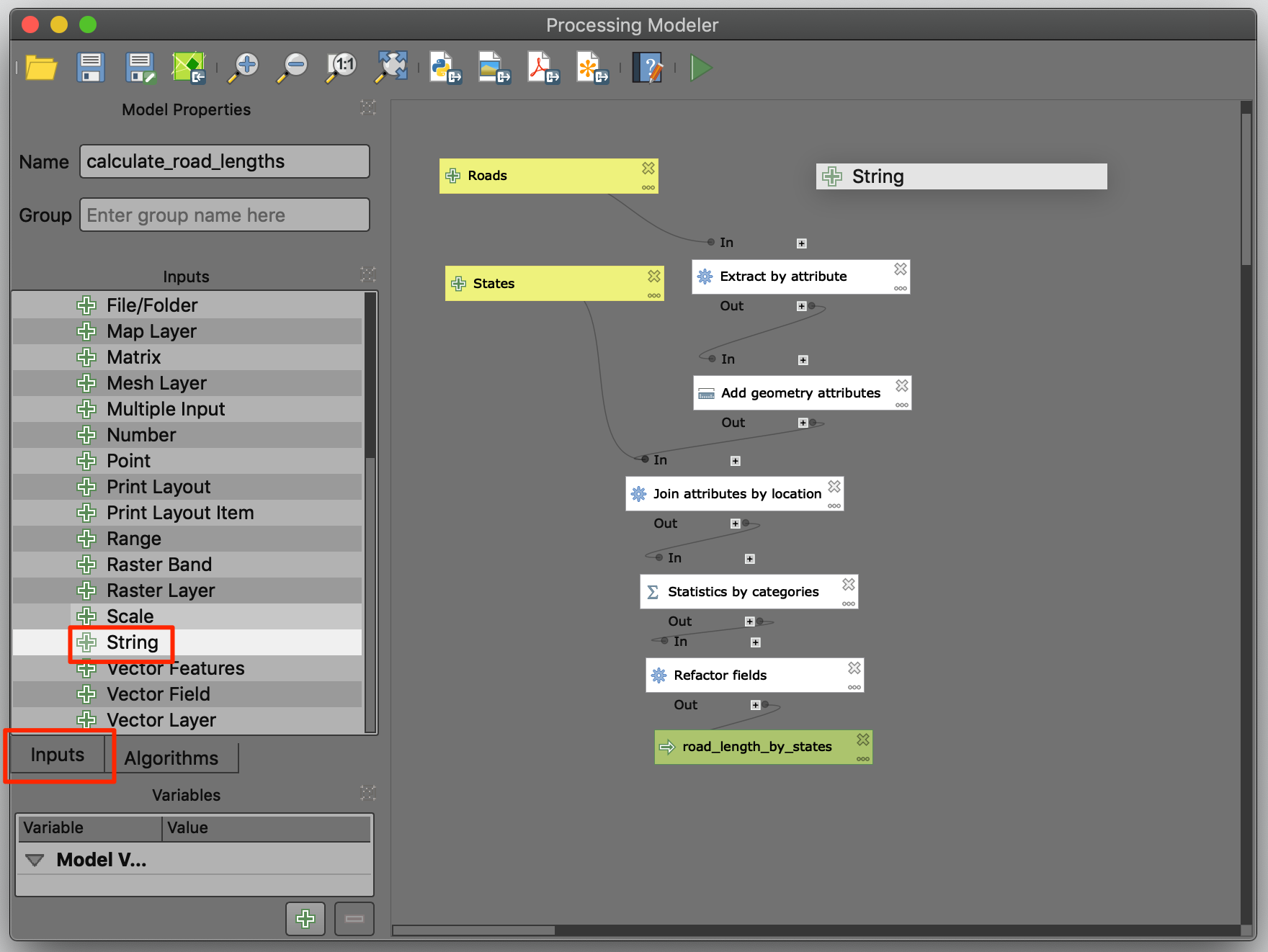
types of roads as well. Go back to the modeler window. Switch to the
Inputs tab and drag a new String input. Enter
Road Categoryas the Parameter name.
If you closed the modeler window, you can open it again by going to Processing → Toolbox → Models. Locate the
calculate_road_lengthsmodel, right-click and select Edit.
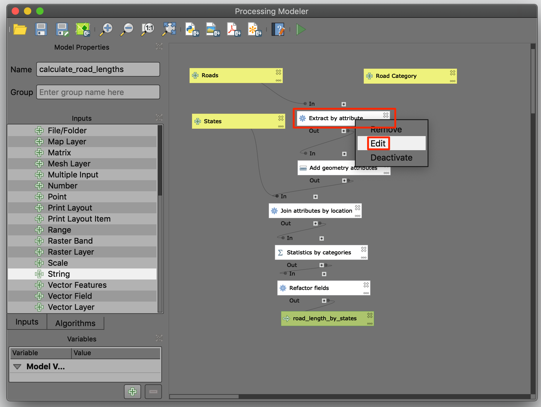
- Now instead of hard-coding the value
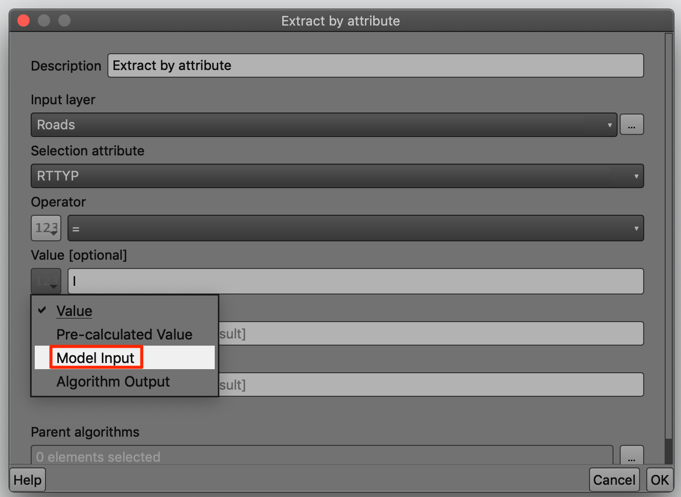
Ifor the road category, we will make it user configurable. Right-click theExtract by attributebox and select Edit.
- Select the 123 button for Value and select
Model Input.
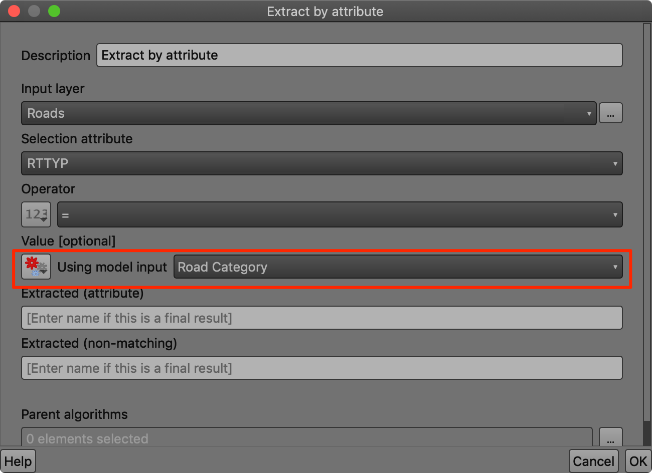
- The parameter
Road Categorywill be auto-selected for the value. This update to our model will allow the user to enter any value as the Road Category which will be used by this algorithm.
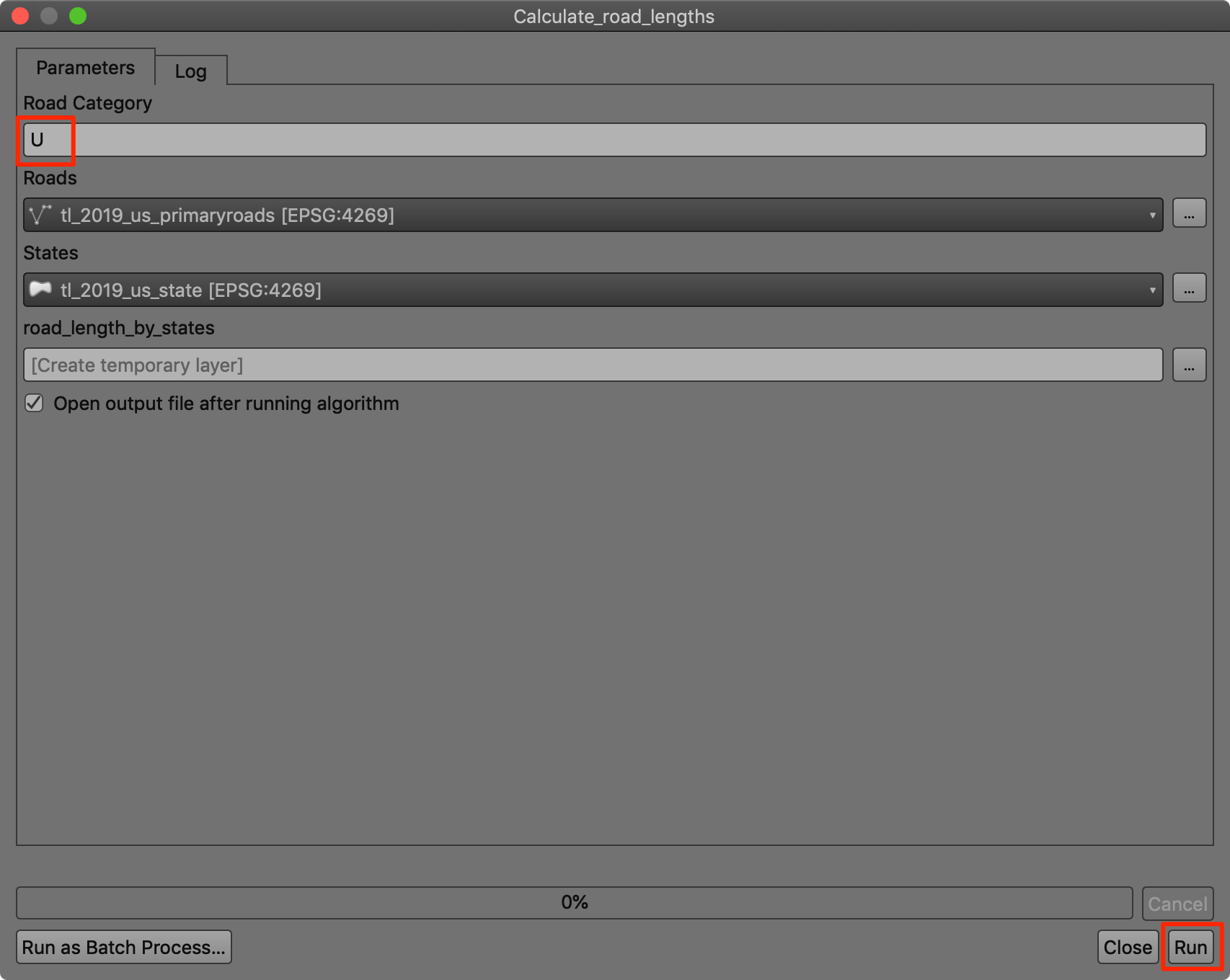
- Let’s test the updated algorithm. Click Run.
- You will see a new input in the model dialog. Enter
Uand select the other vector layer inputs. Click Run. The result will be a table with lengths of US Highways for each state.
Batch Processing
So far we have run the algorithm on 1 layer at a time. But each processing algorithm can also be run in a Batch mode on multiple inputs. This provides an easy way to process large amounts of data and automate repetitive tasks.
The batch processing interface can be invoked by right-clicking any processing algorithm and choosing Execute as Batch Process.
Exercise: Clip multiple layers to a polygon
We will take multiple country-level data layers and use the batch processing operation to clip them to a state polygon in a single operation.
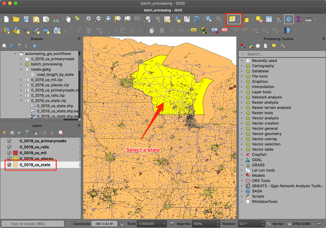
Open the batch_processing project from the data
package. The project contains 5 layers in total. The
tl_2019_us_state represents individual states. The other
layers tl_2019_us_places, tl_2019_us_mil,
tl_2019_us_rails and tl_2019_us_primaryroads
are line and polygon layers which need to be clipped.
- Select the
tl_2019_us_statelayer and use the Select Features tool to select a state by clicking it.
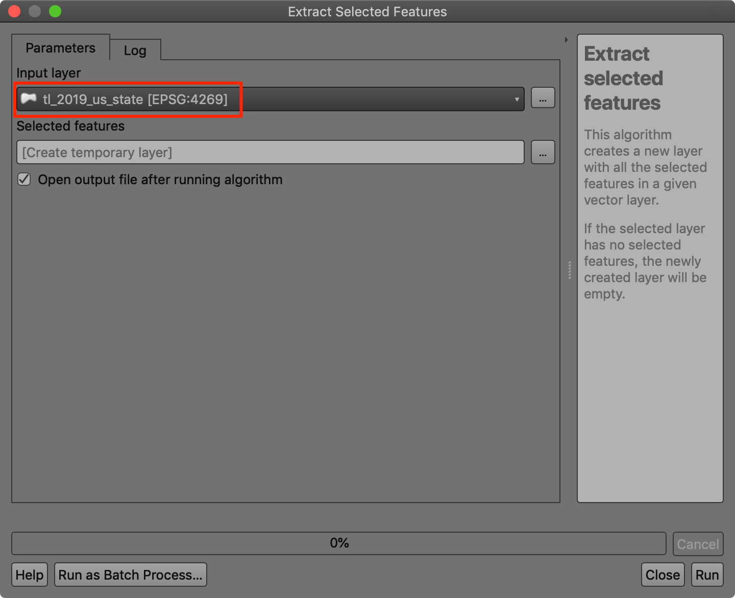
- Next, run the Extract selected features processing
algorithm. Select
tl_2019_us_stateas the Input layer and click Run. This will create a new layer with the selected state polygon calledSelected features
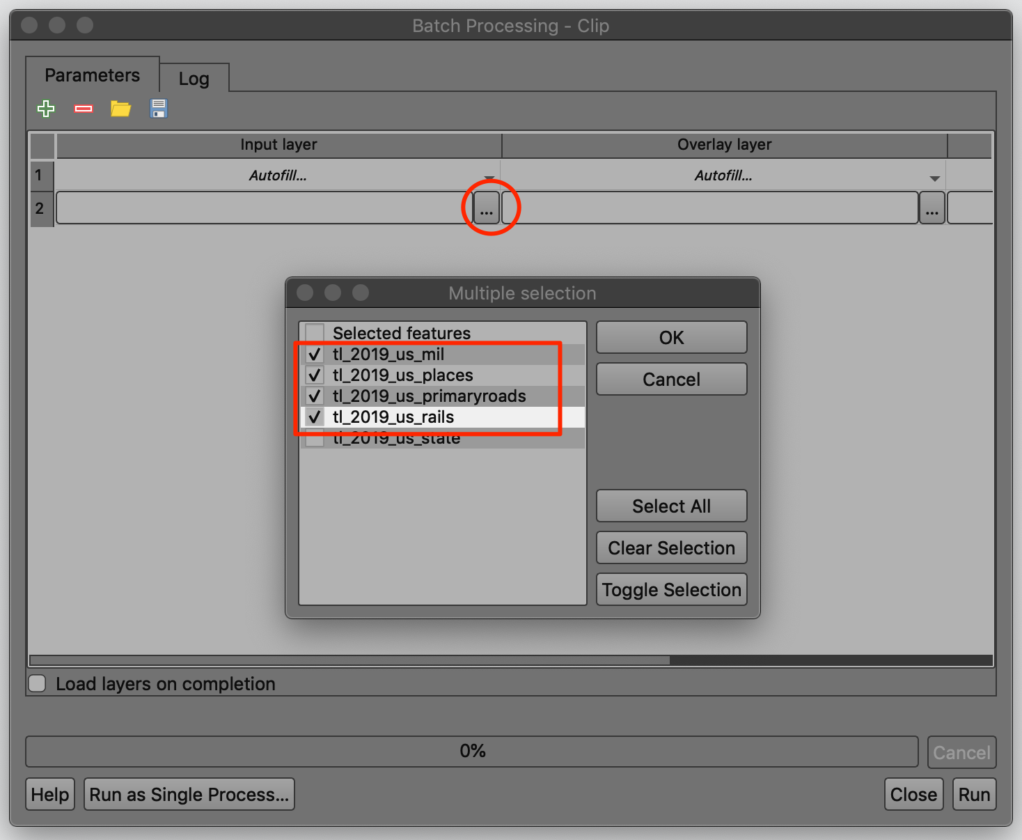
- Search for the Vector Overlay → Clip algorithm and right-click on it. Select Execute as Batch Process.

- In the batch processing dialog, click the … button on the
first row of the Input layer column and choose Select from
Open Layers... Select
tl_2019_us_places,tl_2019_us_mil,tl_2019_us_railsandtl_2019_us_primaryroadslayers and click OK. 3 new rows will be automatically added to accommodate all 4 inputs.
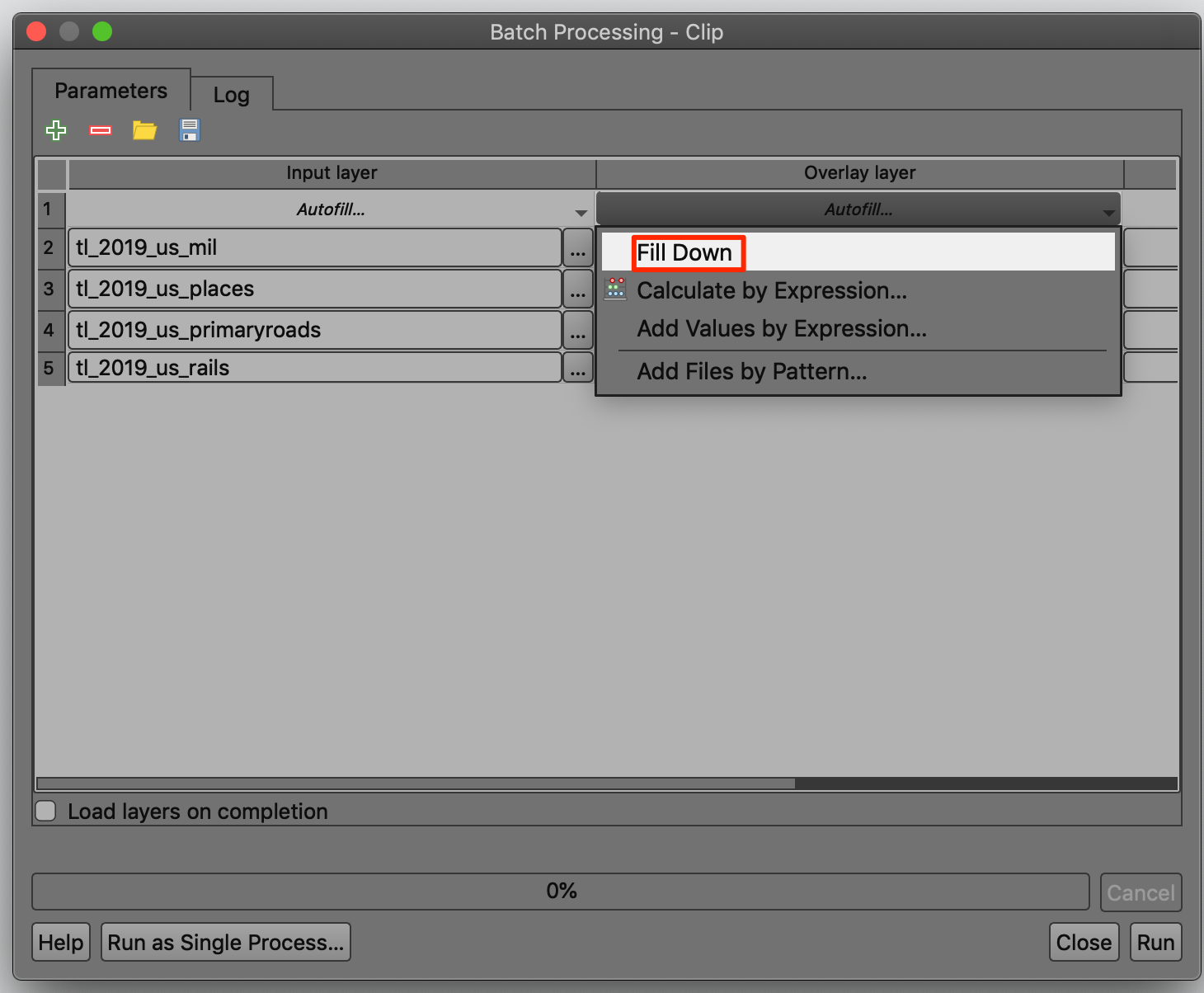
- Click the … button on the first row of the Overlay
layer column. Select the
Selected featureslayer as the Overlay layer.
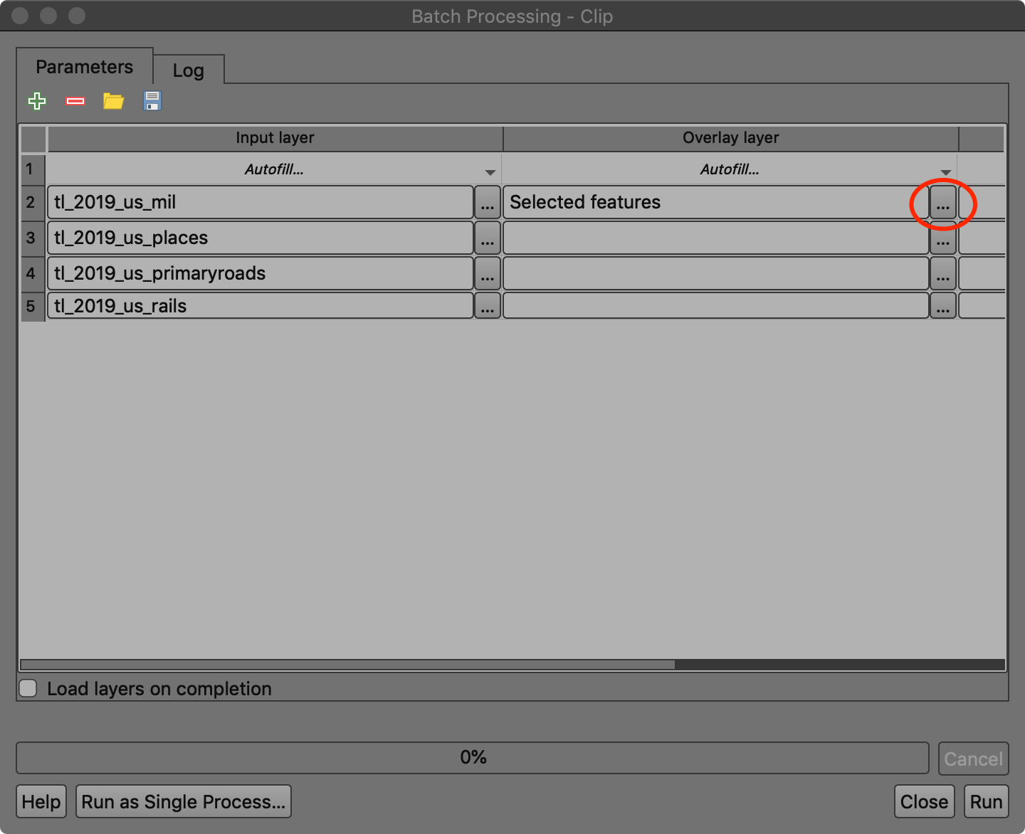
- As all input layers need to be clipped with the same overlay layer, you can click Autofill.. and select Fill Down to autofill all the remaining rows with the same value.
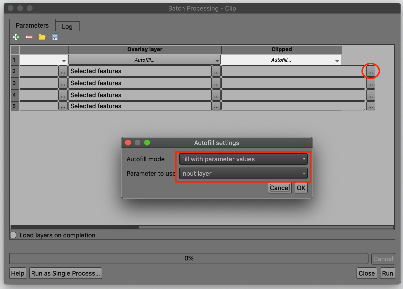
- In the last Clipped column, click the … button and
name the output
clipped_. When prompted, choose Fill with parameter values as the autofill mode, and Input layer as the Parameter to use.
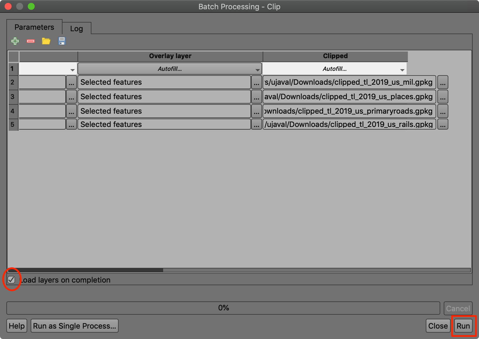
- Make sure the Load layers on completion box is checked and click Run.
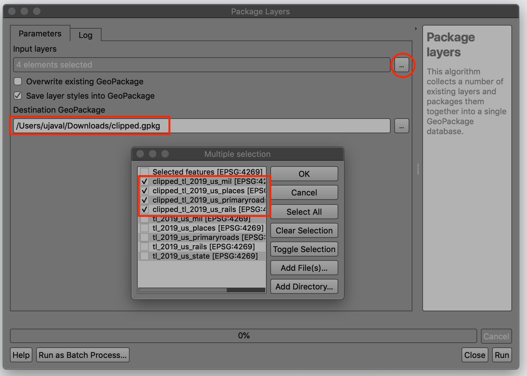
- Resulting clipped layers will be added to the Layers panel. We can combine all the clipped layers into a single geopackage file for ease of sharing. Run the Package Layers processing algorithm.
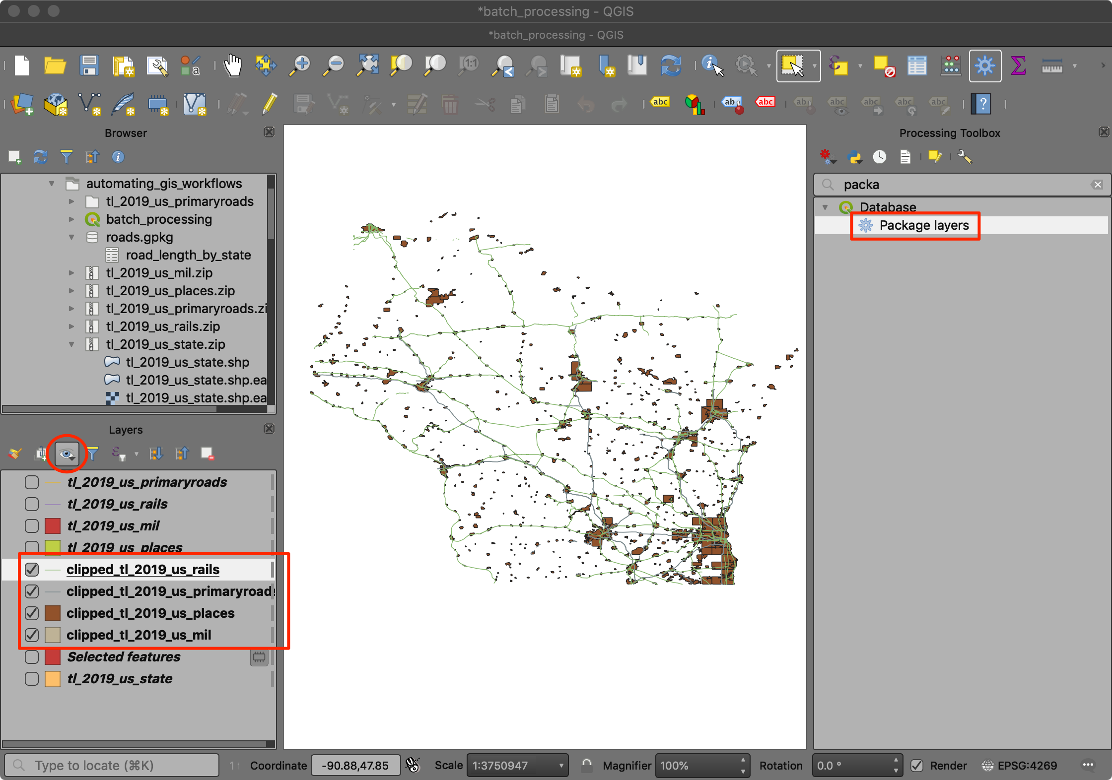
- Choose all the clipped layers and save the output as
clipped.gpkg.
Packaging Your Work
We saw how we can save multiple layers to a single geopackage file. This makes data sharing easy between computers and users. Your spatial analysis project contains a lot more information than the dataset. There are layer styles, settings, variables, processing models etc. that are saved in different places. Modern versions of QGIS have the ability to store all relevant information into a single geopackage. This means you can document your entire project in a single geopackage.
Exercise: Package source layers, results and model in a GeoPackage
We will take the source layers and result of the spatial analysis exercise of finding length of interstate roads and package them up in a GeoPackage.
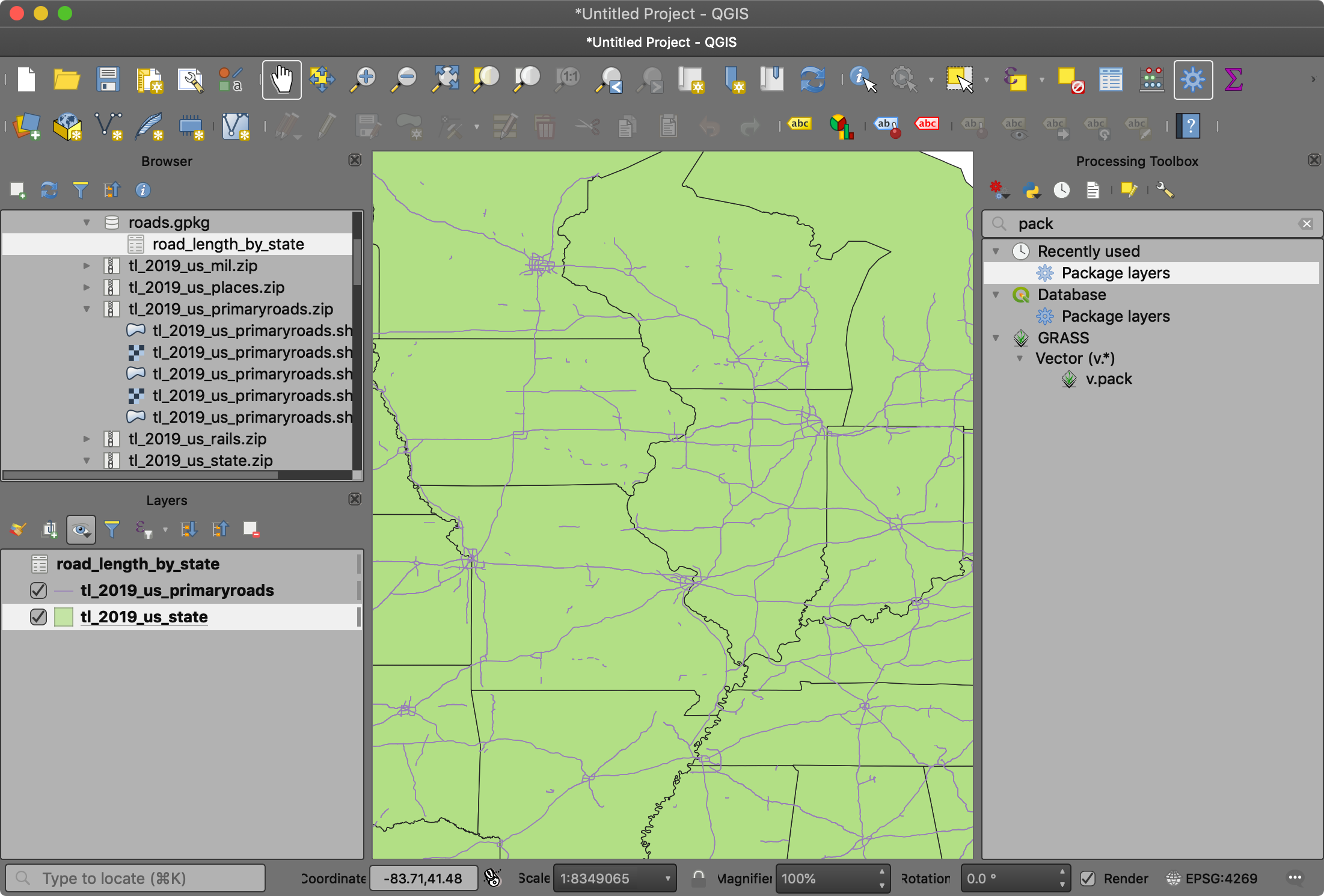
- Load the
tl_2019_us_primaryroads,tl_2019_us_stateandroad_lengths_by_statelayers in QGIS. Run the Package Layers processing algorithm.
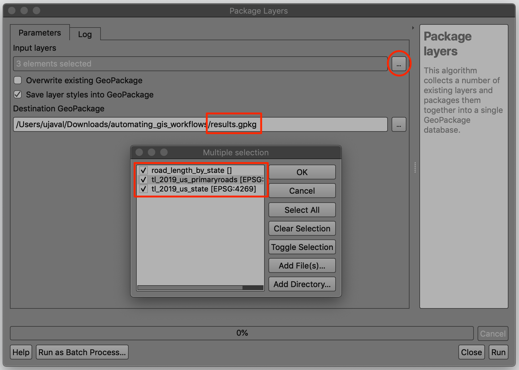
- Choose all the layers as the Input layers. Make sure the
Save layer stles into GeoPackage option is checked. Name the
Destination GeoPackage as
results.gpkg. Click Run.
- Now the layers and their respective layer styles are all contained in a single geopackage file. Click New Project button. You can click Don’t Save when prompted to save the current project.
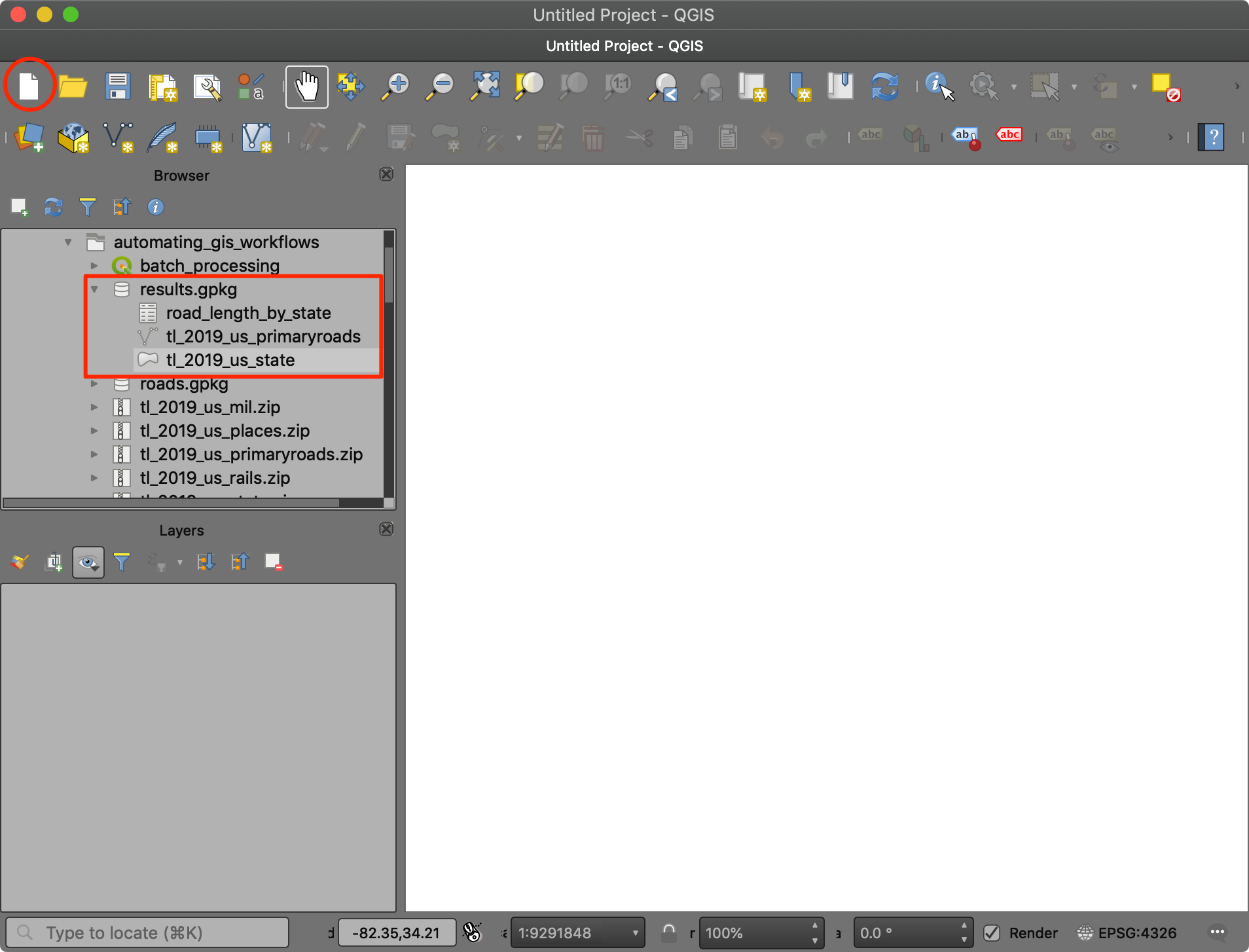
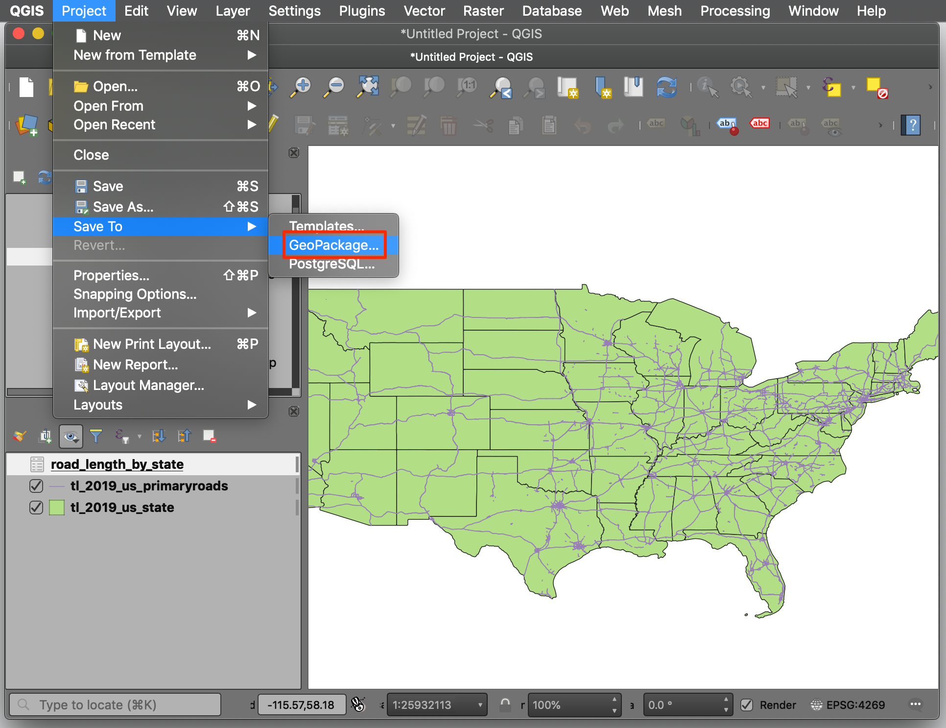
- In the fresh project, drag all the layers from the
results.gpkgback in QGIS. Now that all loaded layers are from a single geopackage, we can save the project. Go to Project → Save To → GeoPackage.
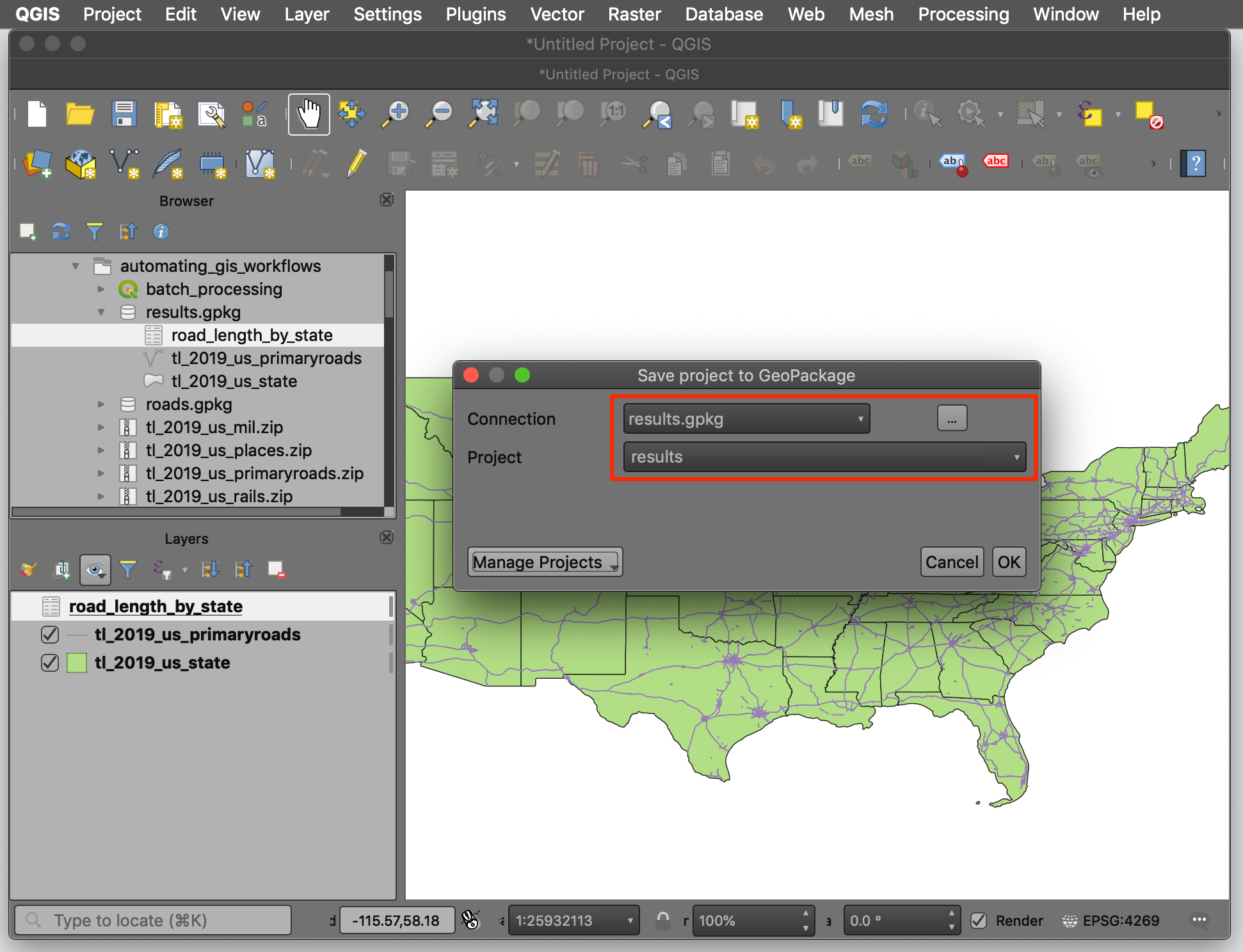
- Click the … button next to Connection and browse
to the
results.gpkgfile. Click OK. Enterresultsas the Project name. Click OK.
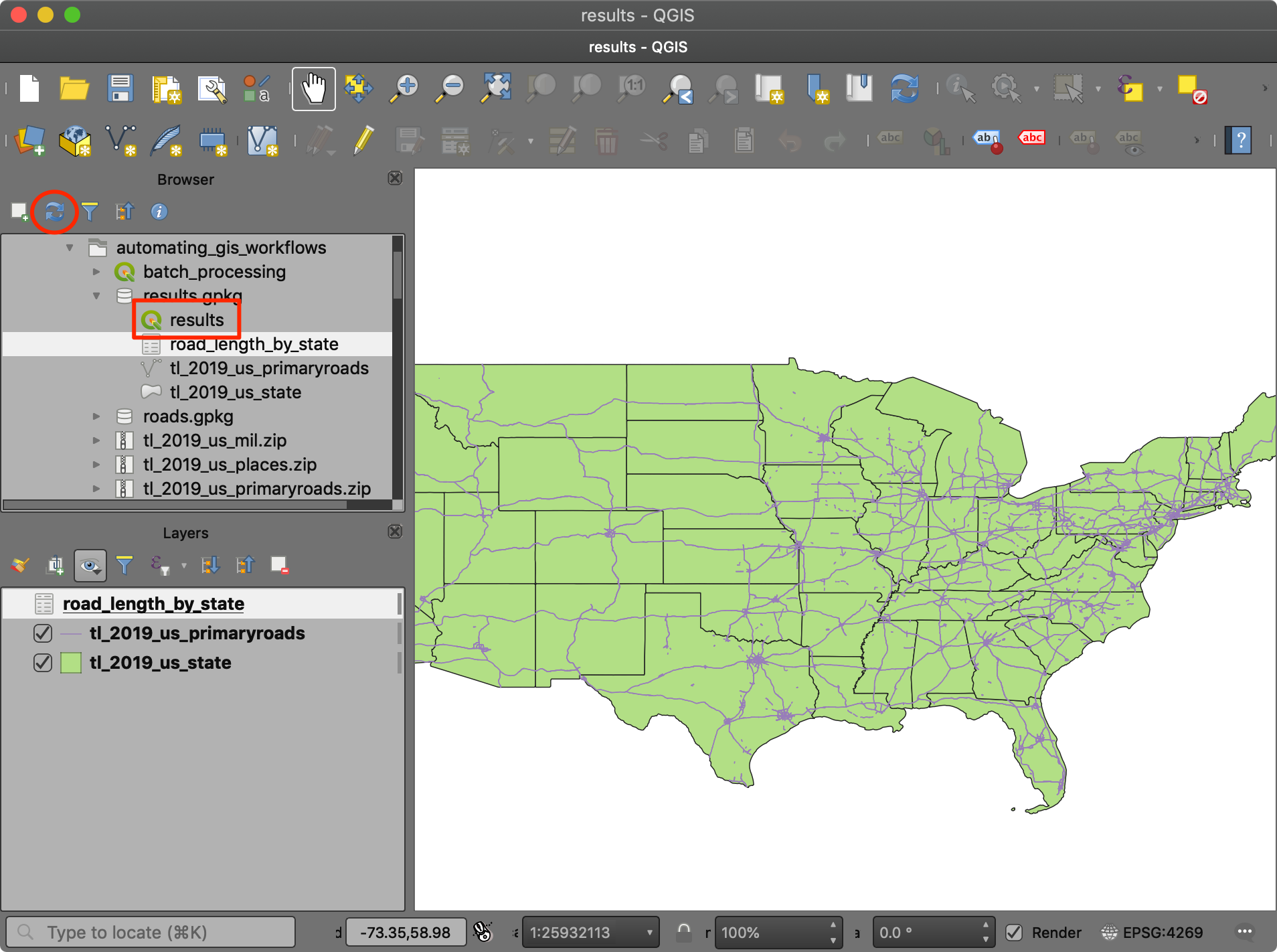
- Now the current project - with its layers, settings, variables etc.
is also saved inside the
results.gpkgfile. Click the Refresh button in the Browser panel and expand theresults.gpkgfile. You will see theresultsproject.
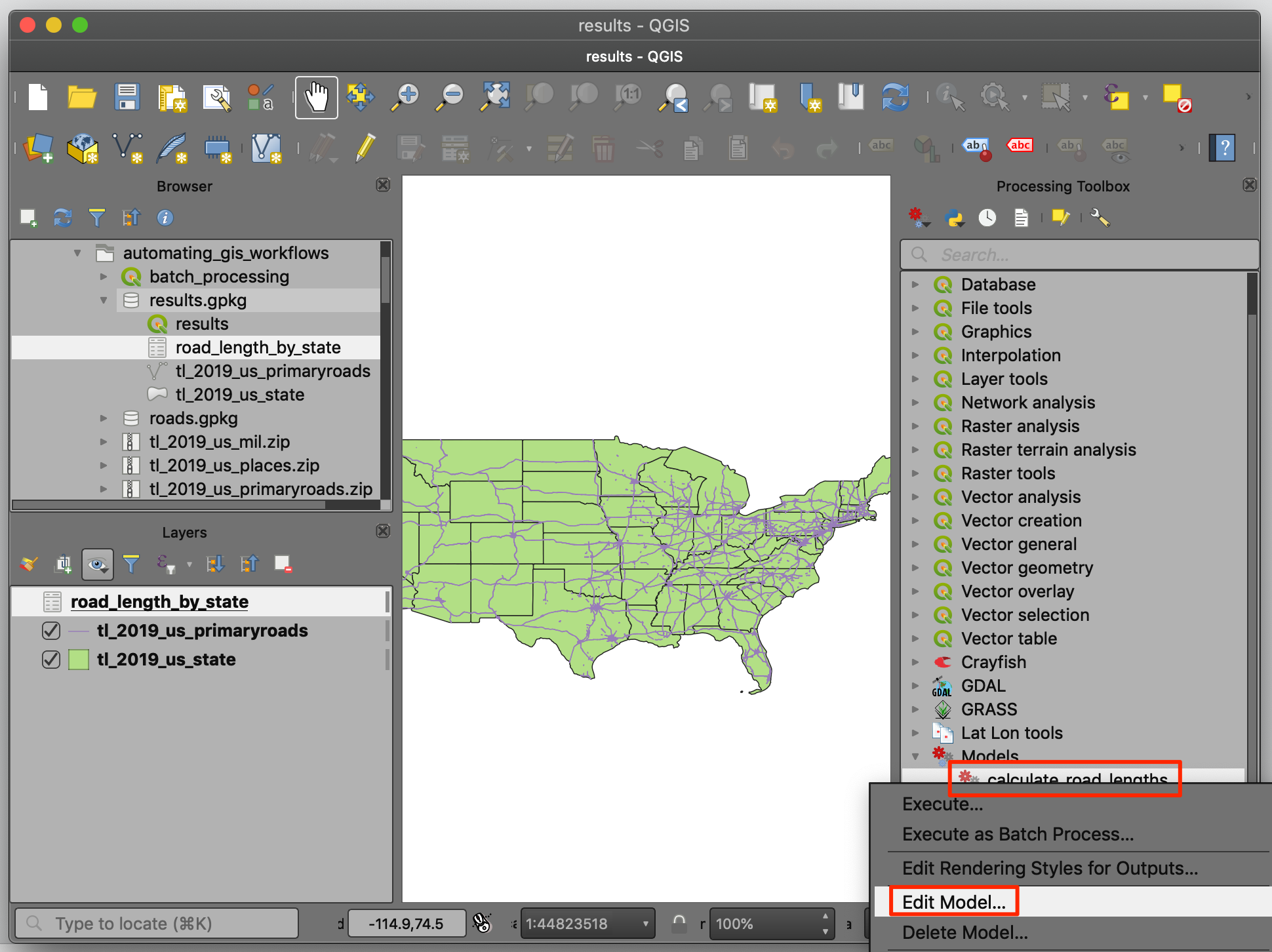
- We can also package our processing model that created the results
inside the package. This is a good practice since anyone who has the
geopackage can reproduce the results using the included model. Open
Processing Toolbox and locate the
calculate_road_lenghtsmodel under Models. Right-click and select Edit Model.
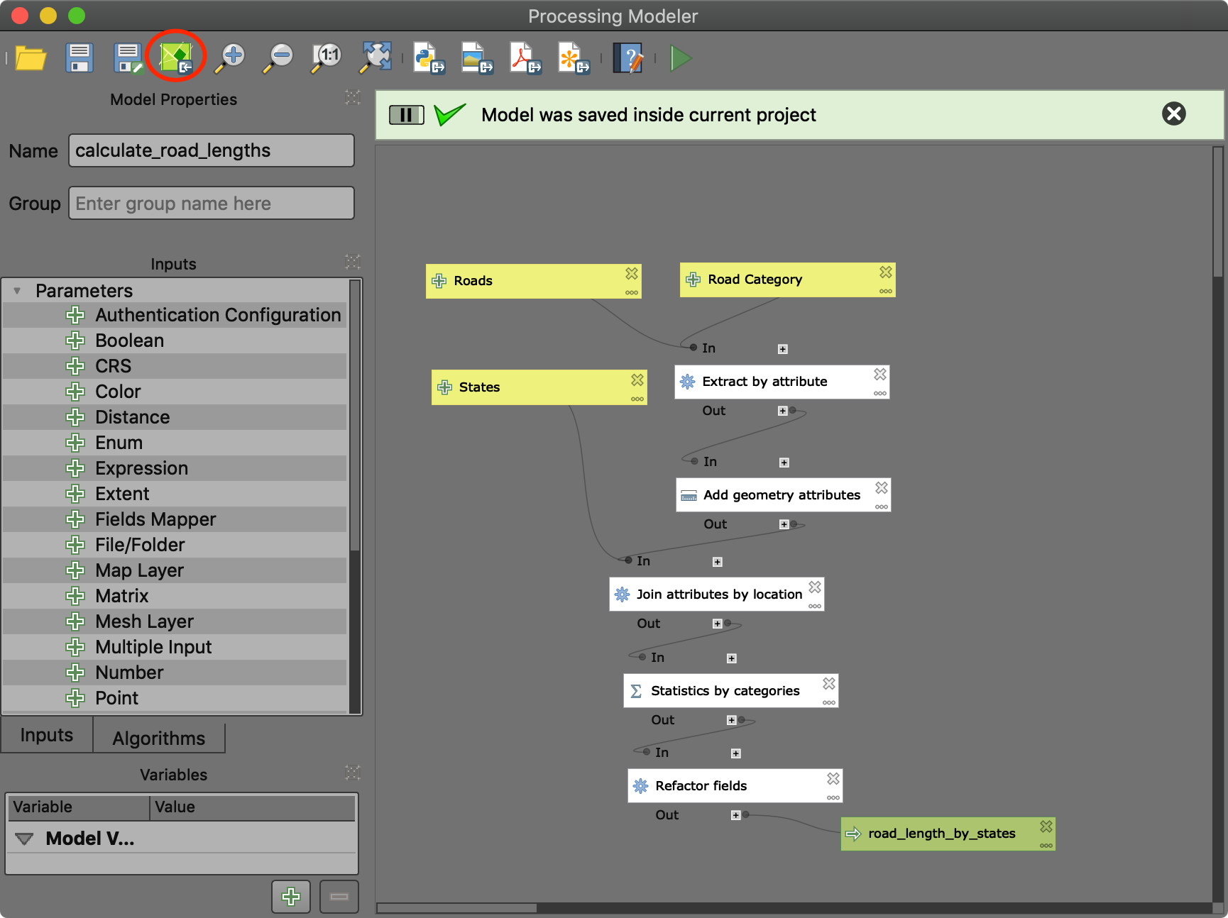
- In the Processing Modeler toolbar, click the Save model in project button. You will get a success message confirming that the model was saved inside the current project.
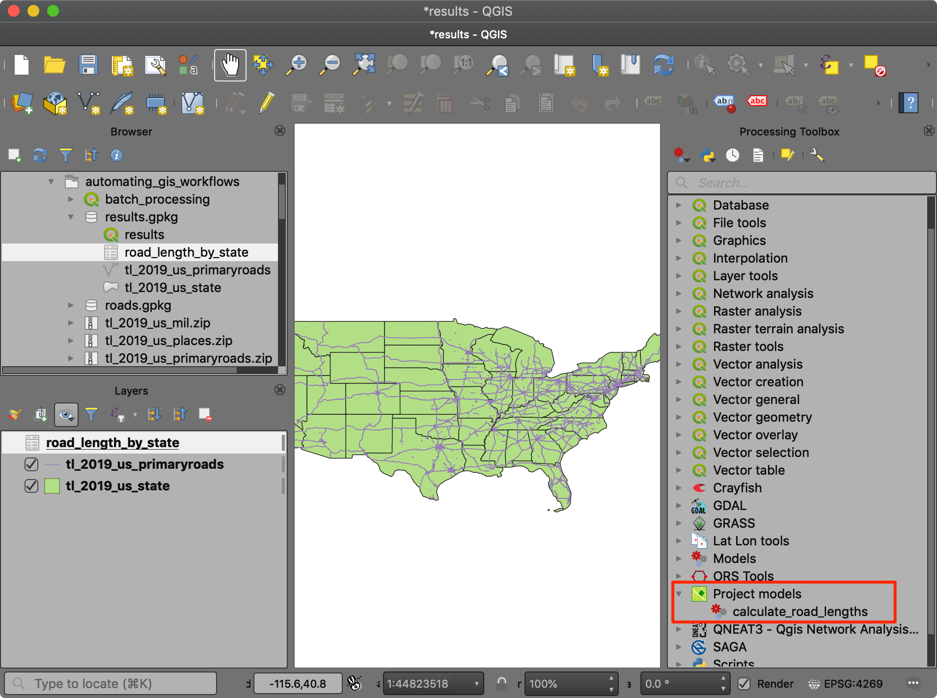
- Back in the main QGIS window, you will see a new section in the Processing Toolbox called Project Models. This folder contains the models that are saved inside the current project. Anyone who opens this project will have this folder and all the models within it.
GeoPackage is a flexible and versatile format that is adopted across QGIS. You saw how you can package all relevant information about your project inside a single file. Following these practices of saving your models along with source data ensures no information is lost. It also ensures you have well documented workflows that are reproducible by you in the future or by anyone with whom you have shared your data.
Data Credits
- TIGER/Line Shapefiles 2019, US Census Bureau.
- Cartographic Boundary Files 2018 for US States, US Census Bureau.
License
This workshop material is licensed under a Creative Commons Attribution 4.0 International (CC BY 4.0). You are free to re-use and adapt the material but are required to give appropriate credit to the original author as below:
Automating GIS Workflows with QGIS by Ujaval Gandhi www.spatialthoughts.com
If you want to report any issues with this page, please comment below.