QGIS Expressions Masterclass (Workshop Material)

Learn QGIS expressions from the ground up.

---

---

Introduction

Expressions are one of the most powerful features of QGIS. In this hands-on workshop, we will start from the basics of expression syntax and you will learn how to solve complex problems by combining the basic building blocks.

This workshop requires basic working knowledge of QGIS.

View the Presentation ↗

Software

This workshop requires QGIS LTR version 3.40.

Please review QGIS-LTR Installation Guide for step-by-step instructions.

Get the Data Package

The code examples in this workshop use a variety of datasets. All the required layers, project files etc. are supplied to you in the zip file qgis-expressions.zip. Unzip this file to the Downloads directory.

The data package also comes with a solutions folder that contains model solutions for each section.

Download qgis-expressions.zip.

1. Operators and Conditionals

In this section, we will learn about operators and conditions used in QGIS expressions and learn how to use them to select and extract features from layers.

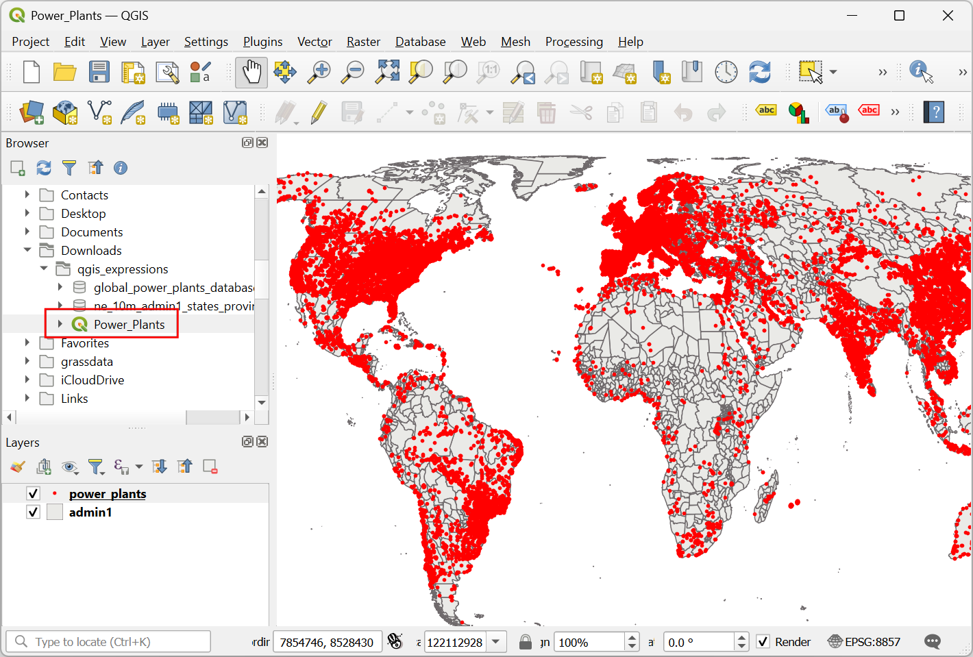
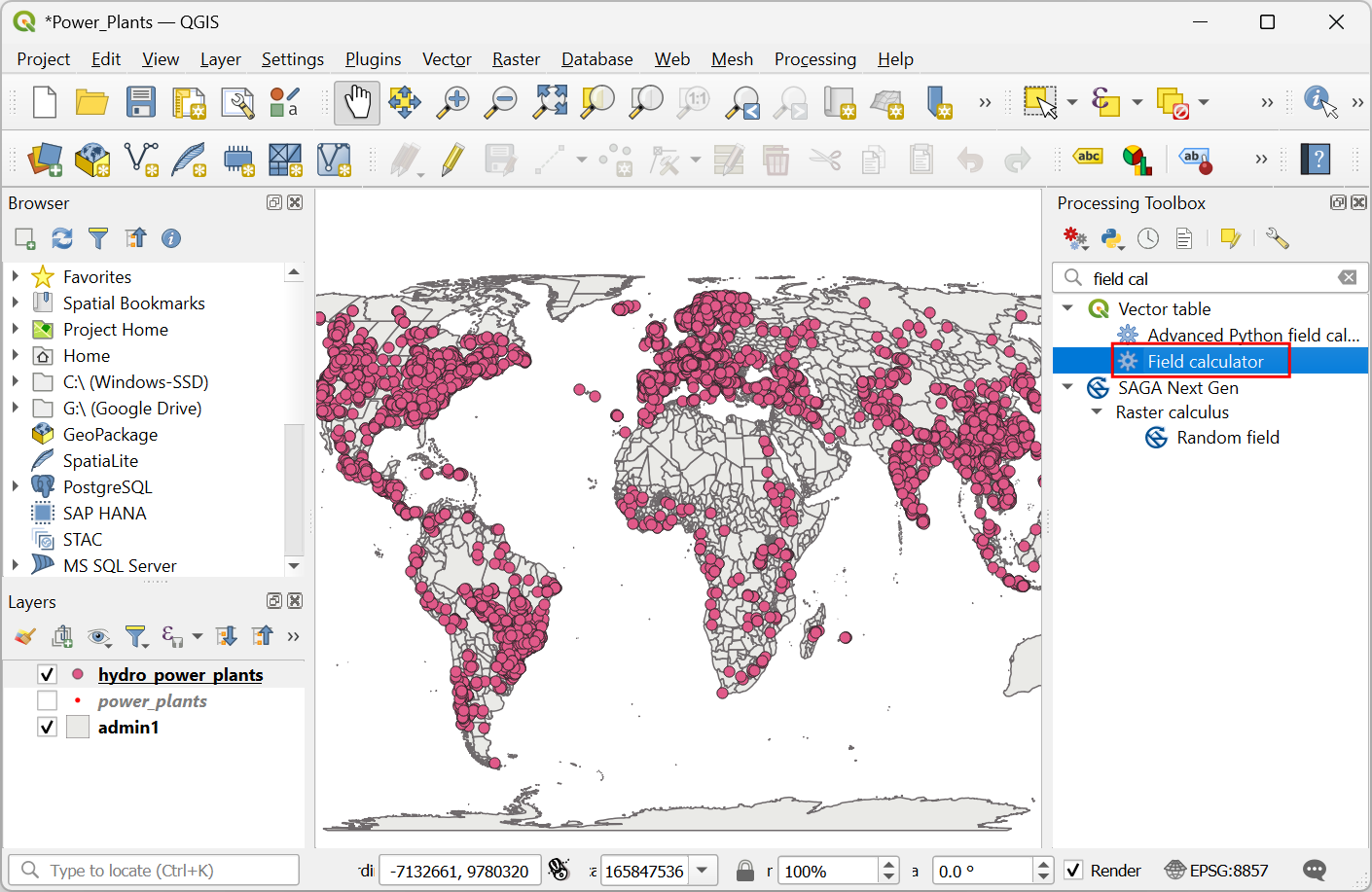
1. Open QGIS. Navigate to the folder containing the data package. Locate and open the Power_Plants project. This project contains 2 data layers. A point layer named power_plants containing locations of all power plants in the world and a polygon layer named admin1 with states/province boundaries for all countries.

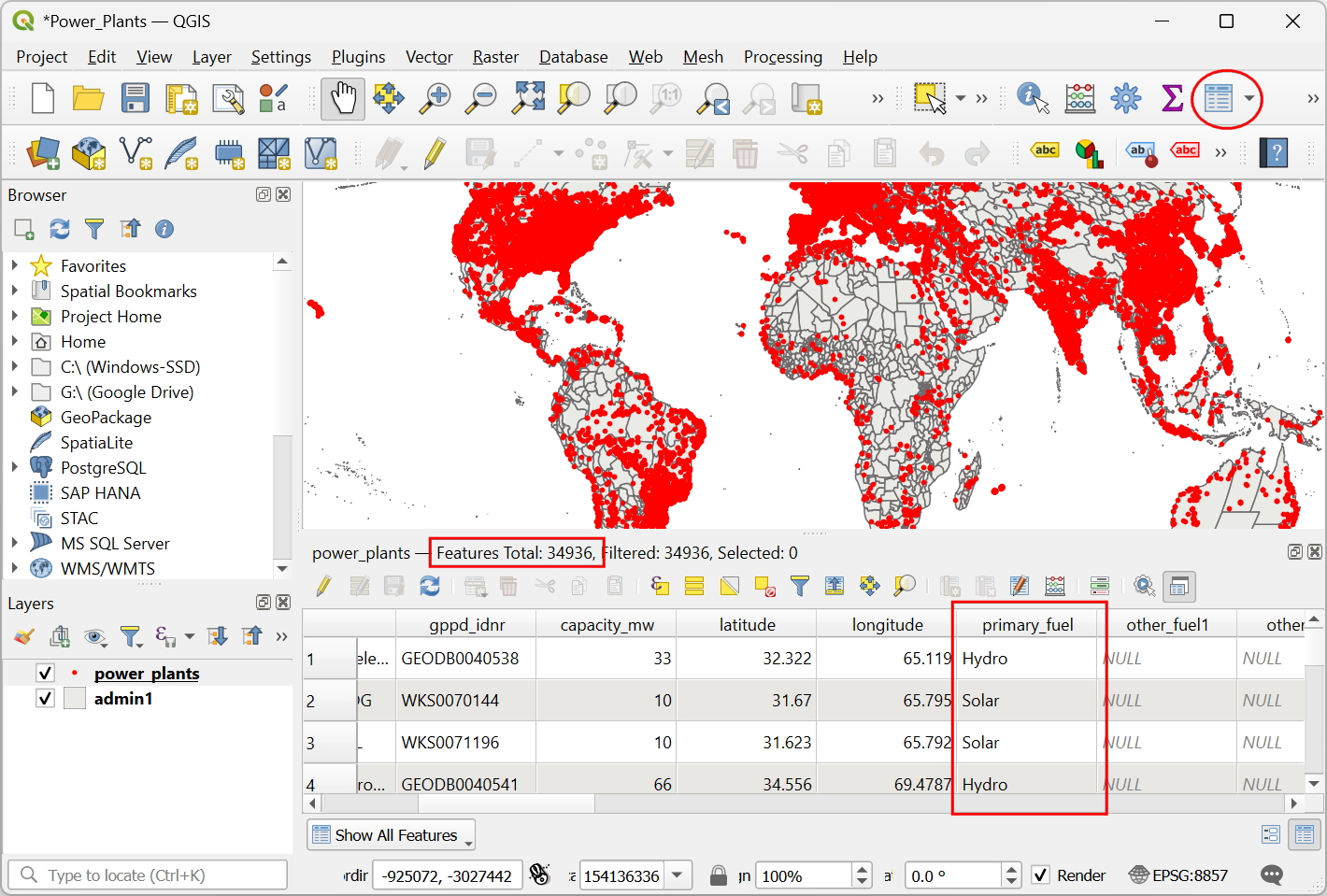
2. Select the power_plants layer and click Open Attribute Table button. You will see that the layer as a column named primary_fuel describing the primary energy source used in electricity generation. We can use this to select different types of power plants.

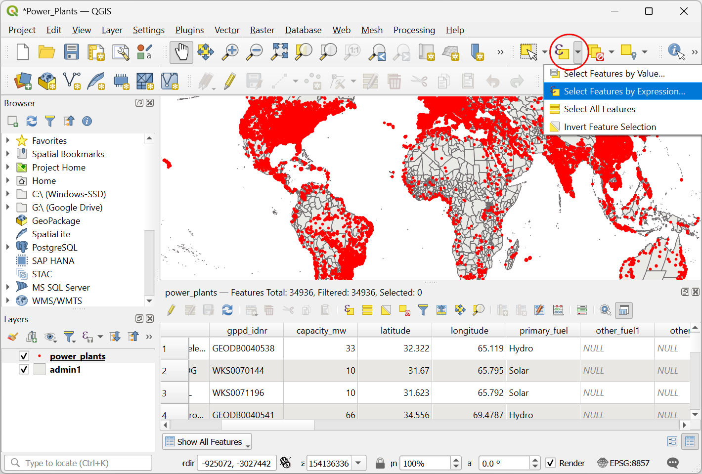
3. We will now use an expressions to select features from this layer. From the Selection Toolbar, click the Select Features by Expression… button.

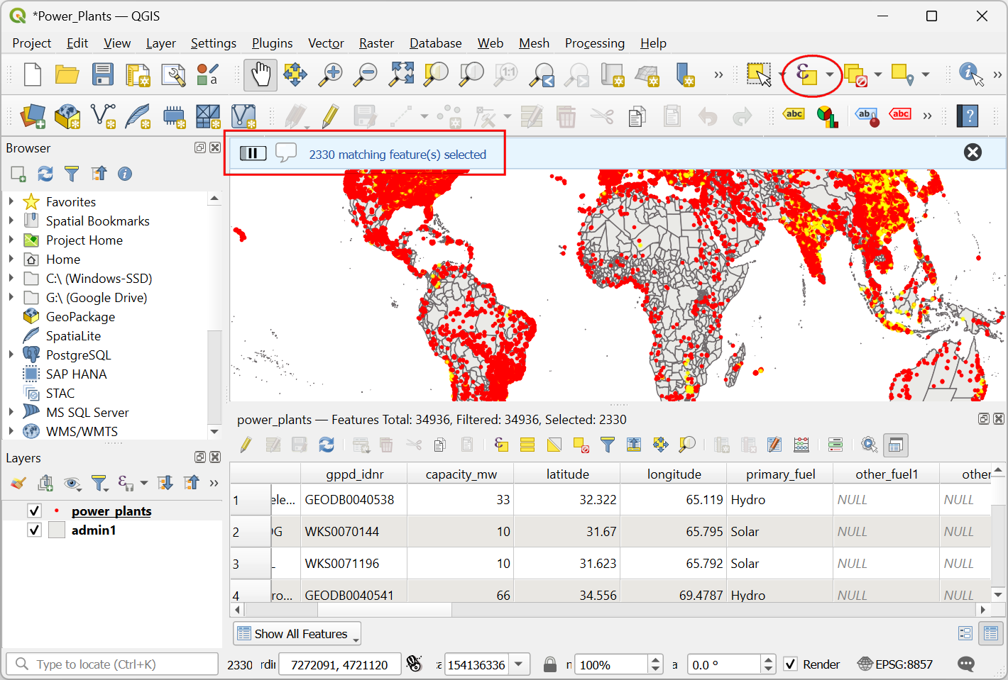
4. In the Expression dialog, locate the primary_fuel attribute under Fields and Values group. Double-click to add it to the expression. While the field is selected, click the All Unique button to show all unique values contained in that field. Here we want to select all Coal power plants, so enter the expression as below and click Select Features.

"primary_fuel" = 'Coal'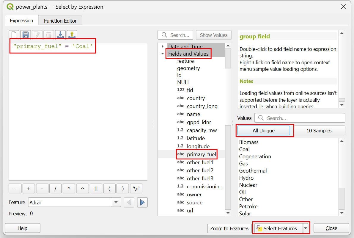

5. In the main QGIS window, you will see the features matching the expression selected in yellow color. We could select all Coal power plants. What if we want to select all power plants that use renewable energy source? We need to be able to specify multiple fuel types for the query. Let’s update the expression. From the Selection Toolbar, click the Select Features by Expression… again.

6. We can use the IN operator to specify a list of fuel types that we want to select. Enter the following expression and click Select Features.

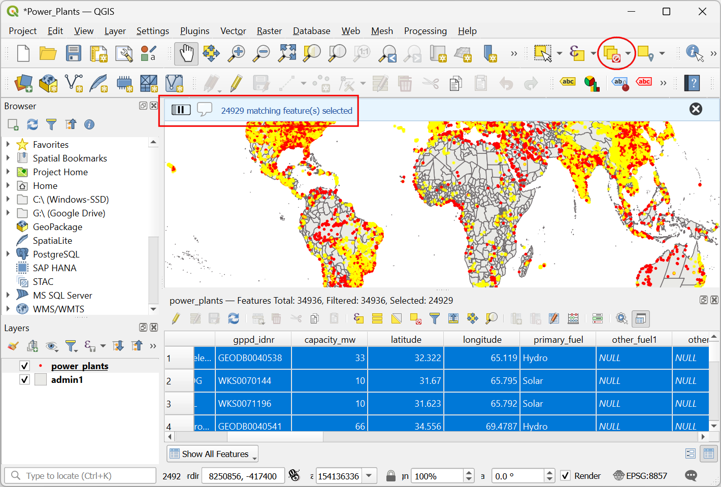
"primary_fuel" IN ('Biomass', 'Geothermal', 'Hydro', 'Solar', 'Wind', 'Storage', 'Wave and Tidal')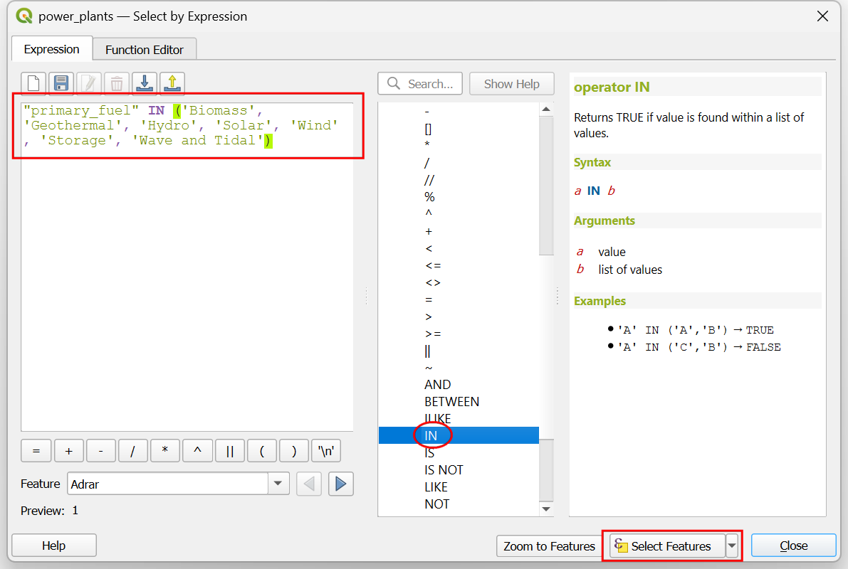

7. You will now see all power plants with renewable fuel types selected. Click the Deselect Features from All Layers button.

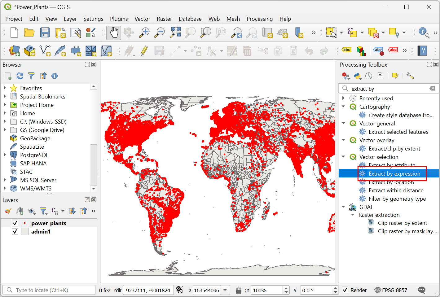
8. Next, we will learn how we can use expressions to extract certain features into a new layer. Open the Processing Toolbox from Processing → Toolbox. Search and locate the algorithm Vector selection → Extract by expression and double-click to launch it.

9. In the Vector Selection - Extract by Expression dialog, select power_plants as the Input layer. Click the Expression button.

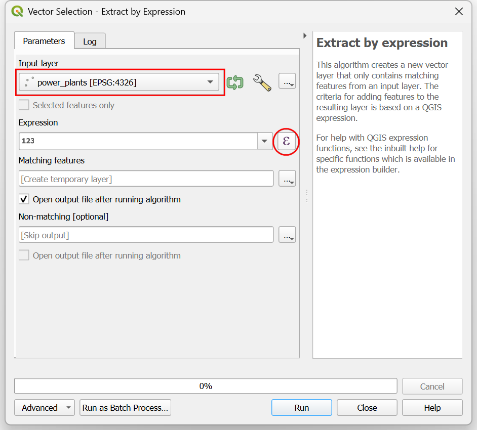
10. Enter the following expression to extract all hydro power plants and click OK.

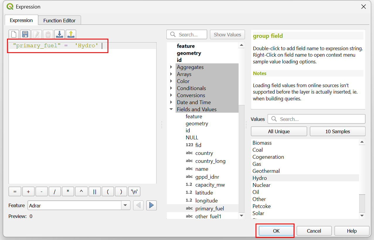
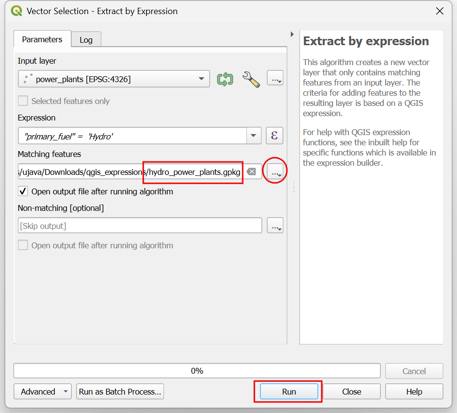
11. Click the … next to Matching Features and select Save to File…. Enter the name of the output file as hydro_power_plants.gpkg and click Run.

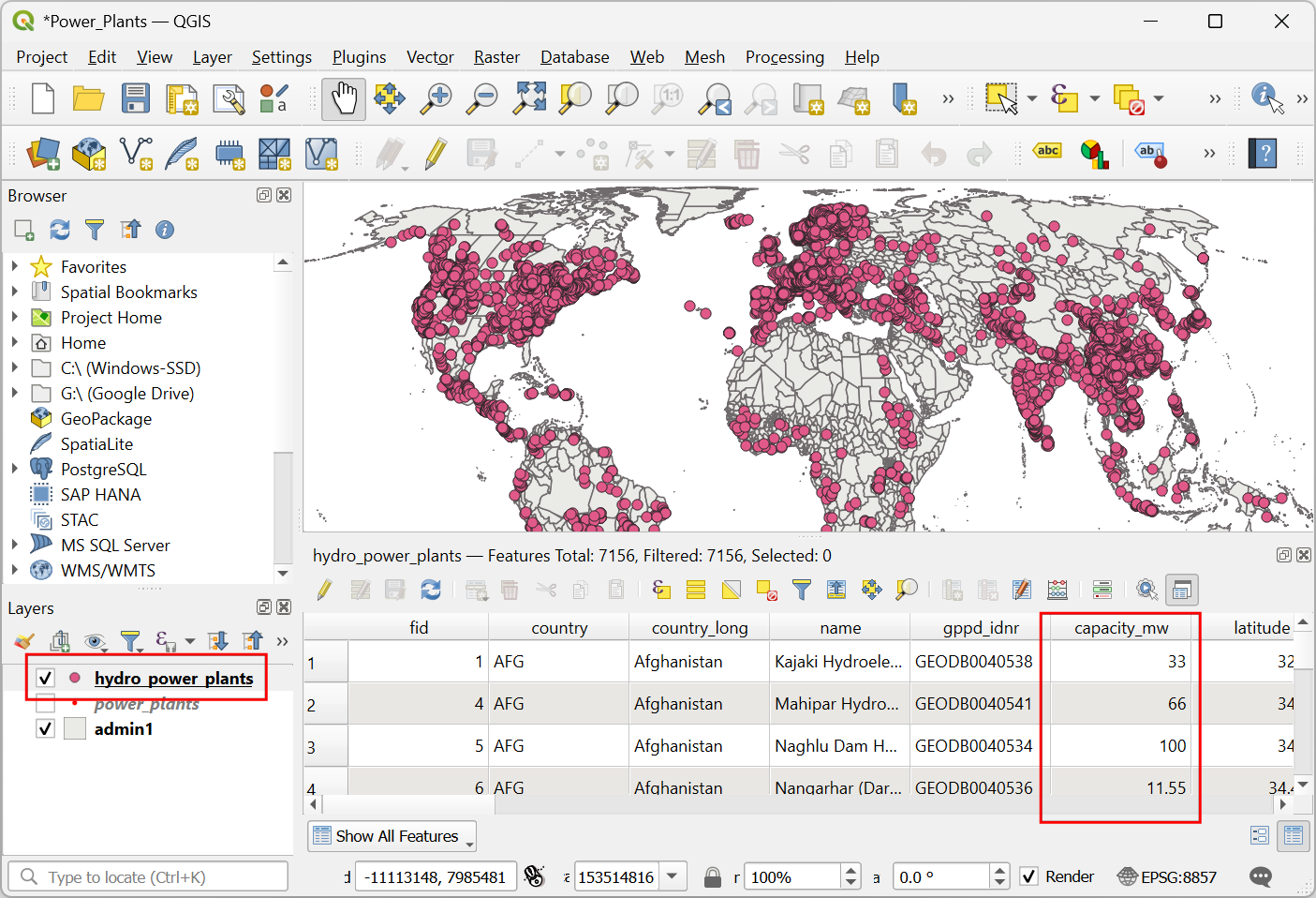
12. Once the processing finishes, a new layer hydro_power_plants will be added to the Layers panel. Open the attribute table and verify that all the power plants have Hydro as the primary_fuel. Next, we will learn how to classify these power plants based on their capacity. The column capacity_mw has electrical generating capacity in megawatts. You may now turn off the visibility of the power_plants layer.

13. Select the hydro_power_plants layer. From the Processing Toolbox, search and locate the algorithm Vector table → Field calculator and double-click to launch it.

14. In the Vector Table - Field Calculator dialog, select hydro_power_plants as the Input Layer. Enter classification as the Field name. Keep Text (string) as the Result field type.

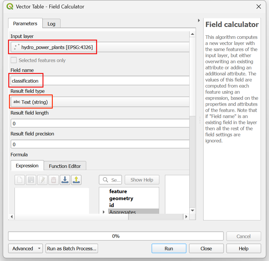
15. We want to assign one of the categories from Small, Medium and Large to each power plant based on the capacity. We can use the CASE statement to assign different values based on different conditions. Enter the following expression.

CASE
WHEN  "capacity_mw" < 25 THEN 'Small'
WHEN  "capacity_mw" >= 25 AND  "capacity_mw" <= 100 THEN 'Medium'
WHEN  "capacity_mw" > 100 THEN 'Large'
END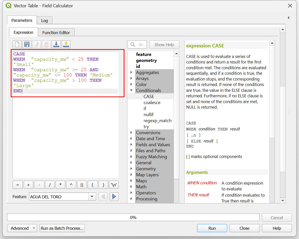

16. Click the … next to Calculated and select Save to File…. Enter the name of the output file as hydro_power_plants_classification.gpkg and click Run.

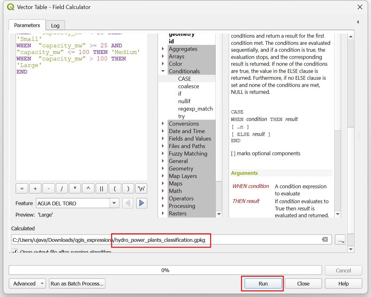
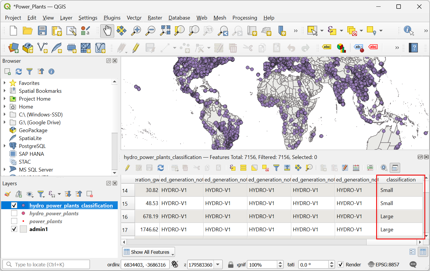
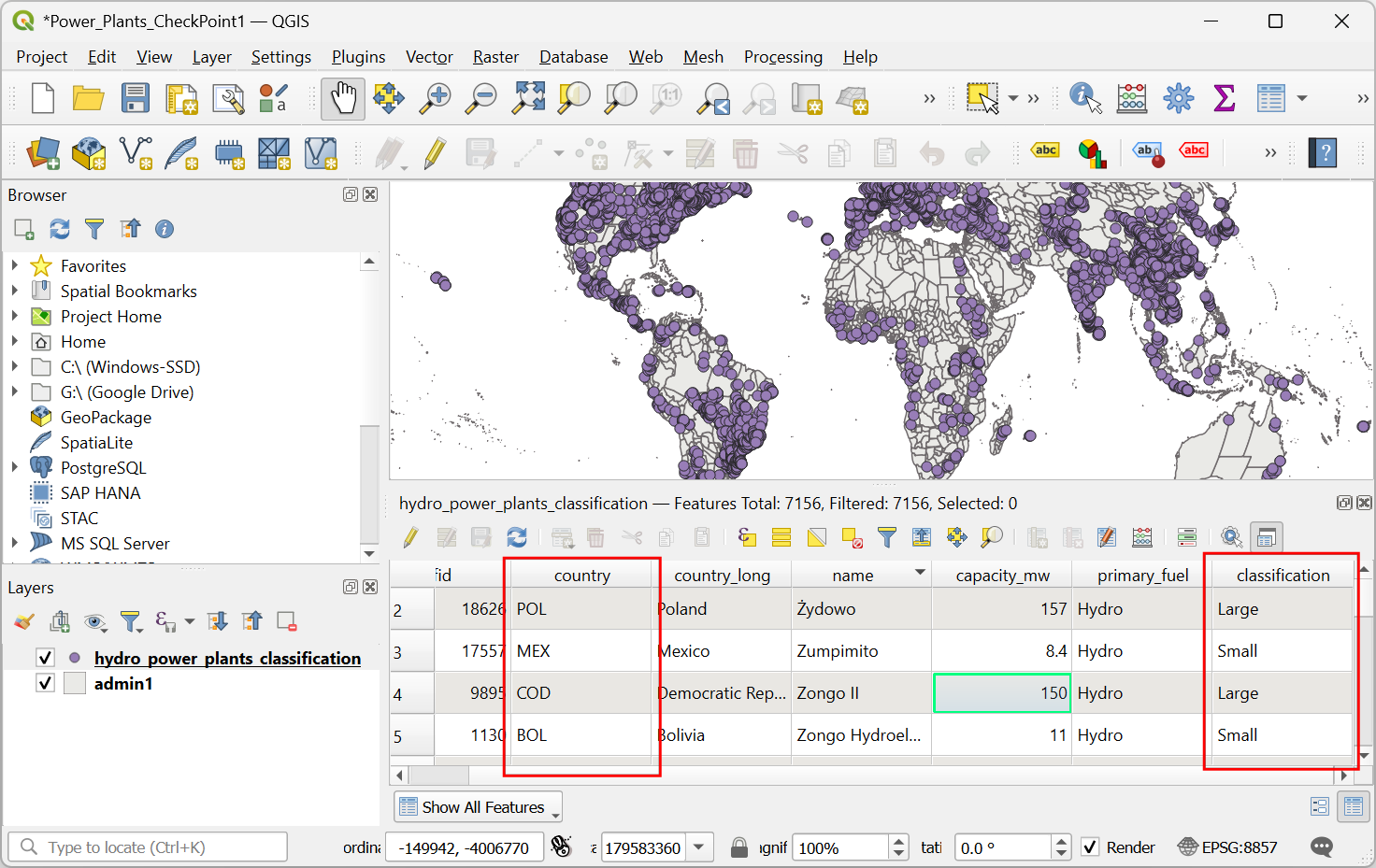
17. Once the processing finishes, a new layer hydro_power_plants_classification will be added to the Layers panel. Open the attribute table and see the assigned values in the classification column.

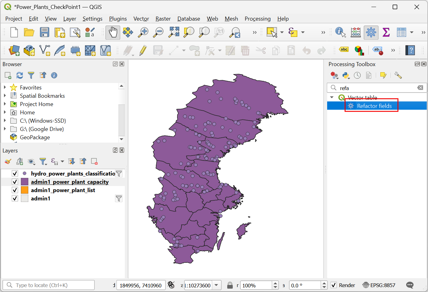
We have now finished the first part of this exercise. You can load the Power_Plants_CheckPoint1.qgz project in the solutions folder to catch up to this point and do the challenge.

Challenge 1

Create a new layer containing only the Large hydro power plants in your country. The country column contains 3-digit ISO codes for each country. Pick a country and build an expression to extract the features.

2. Functions

We will now learn how to use the expression functions for spatial analysis. Our goal will be to get a list of hydro power plants and the total installed capacity for each admin1 region in a country.

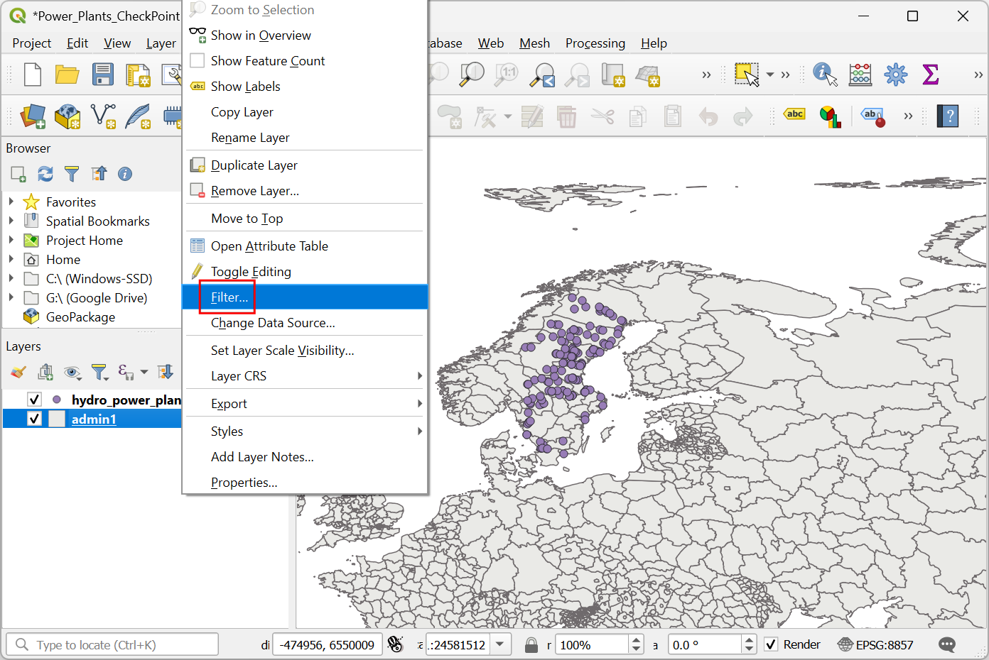
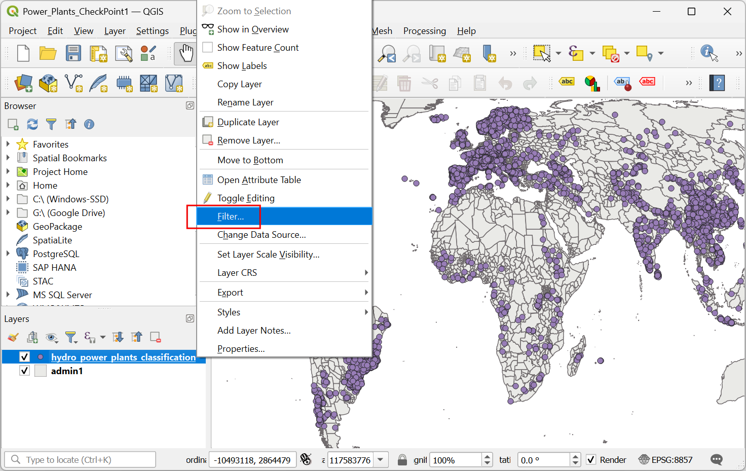
1. Continuing from the previous section, remove all layers except the admin1 and hydro_power_plants_classification layers. We will now apply a filter to each of these layers to keep only the features for our chosen country. Right=click the hydro_power_plants_classification layer and choose Filter….

2. In the Query Builder dialog, enter the following expression and click OK. You may replace SWE with the 3-digit ISO code for your country.

"country" = 'SWE'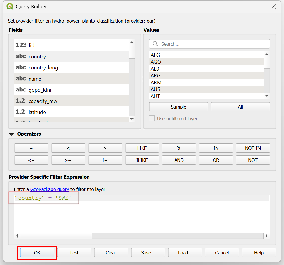

3. Next, right-click the admin1 layer and select Filter….

4. In the Query Builder dialog, enter the following expression and click OK.

"adm0_a3" = 'SWE'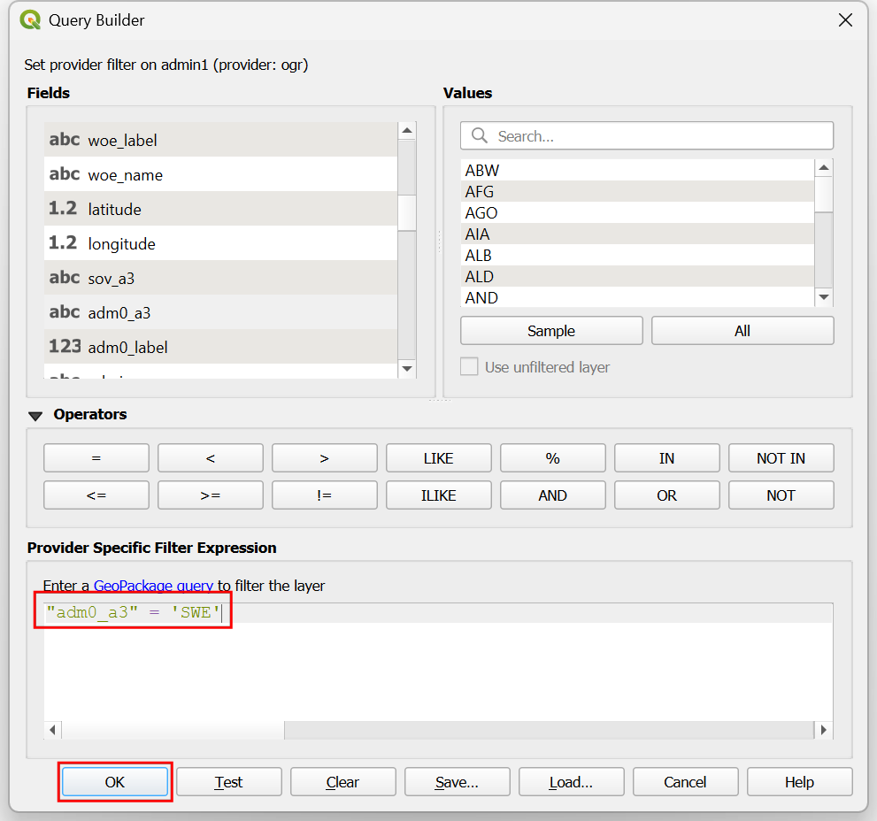

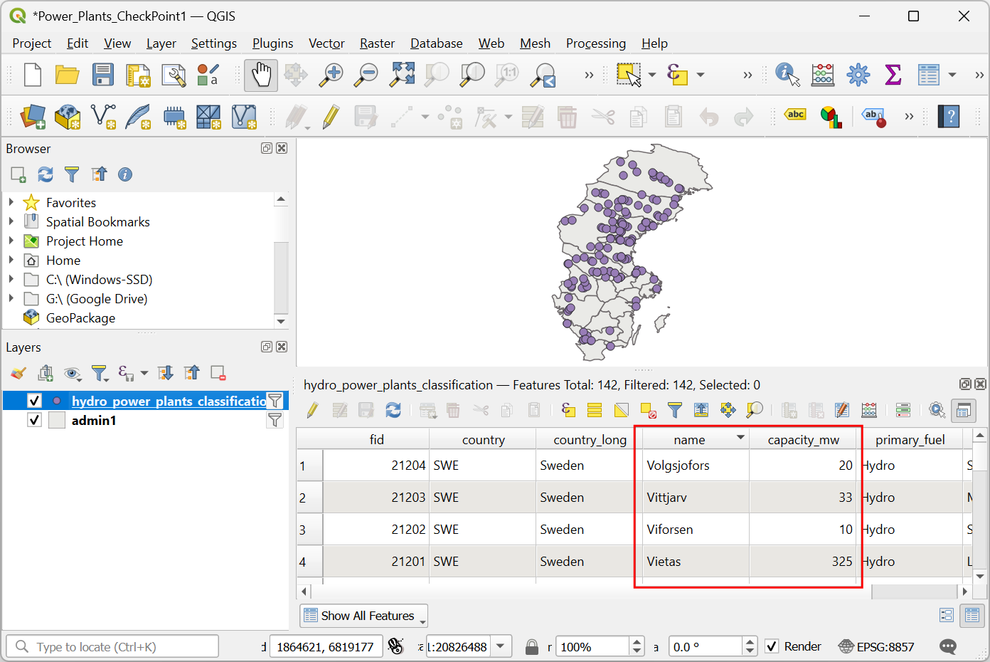
5. Both the layers now have an active filter applied to them and you should only see features for the chosen country. Select the hydro_power_plants_classification layer and open the Attribute Table. Note that the column name contains the name of the power plant and the column capacity_mw contains the power generation capacity.

6. Select the admin1 layer and open the Processing Toolbox from Processing → Toolbox. Search and locate the algorithm Vector table → Field calculator and double-click to launch it.

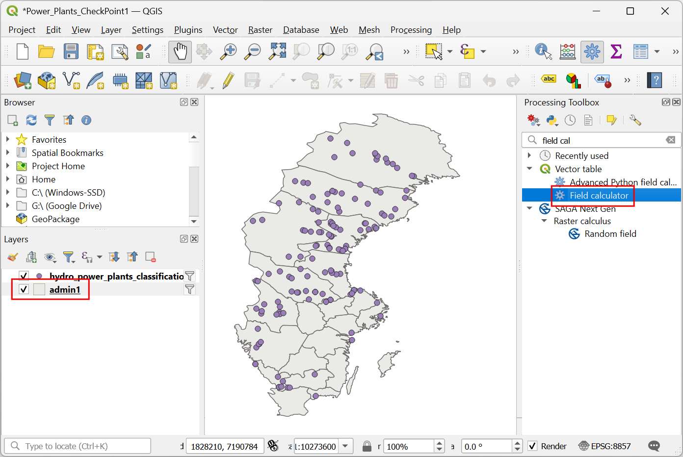
7. In the Vector Table - Field Calculator dialog, select admin1 as the Input Layer. Enter power_plants_list as the Field name. Select String List as the Result field type.

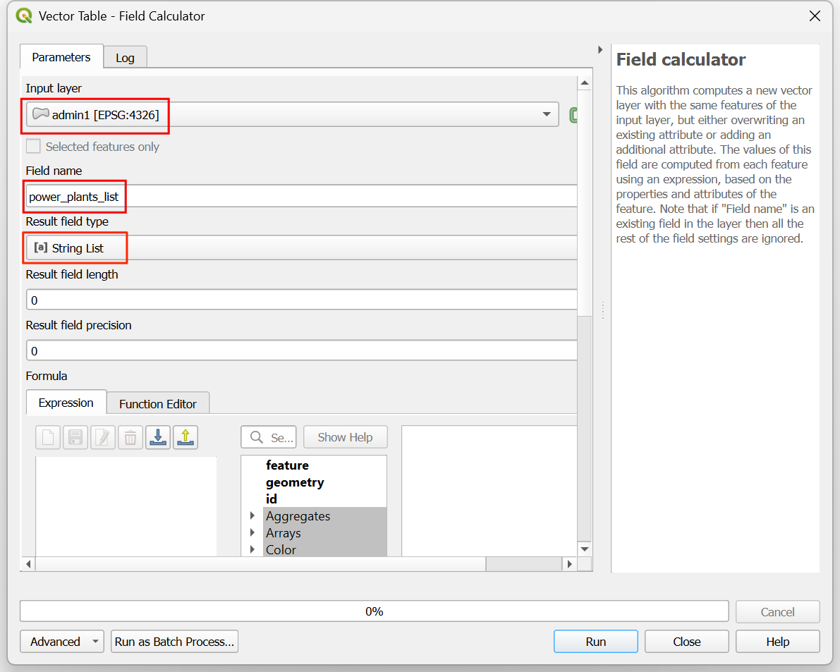
8. We want to find the names of all power plant features intersecting each admin1 polygon. The overlay_intersect() function allows you to locate intersecting features from another layer. Enter the following expression.

overlay_intersects(
  layer:='hydro_power_plants_classification',
  expression:="name"
)

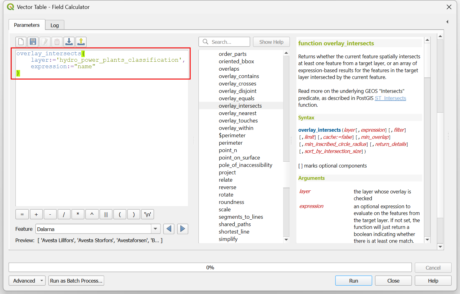
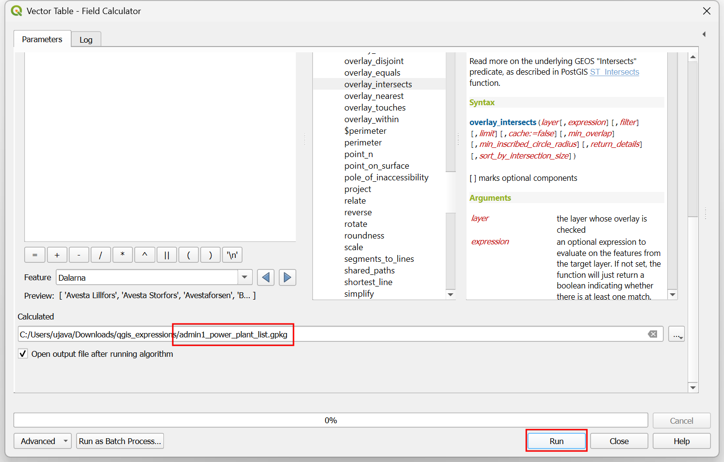
9. In the Preview below the expression, you can see the output is a list of matching power plants for admin1 region. Click the … next to Calculated and select Save to File…. Enter the name of the output file as hydro_power_plant_list.gpkg and click Run.

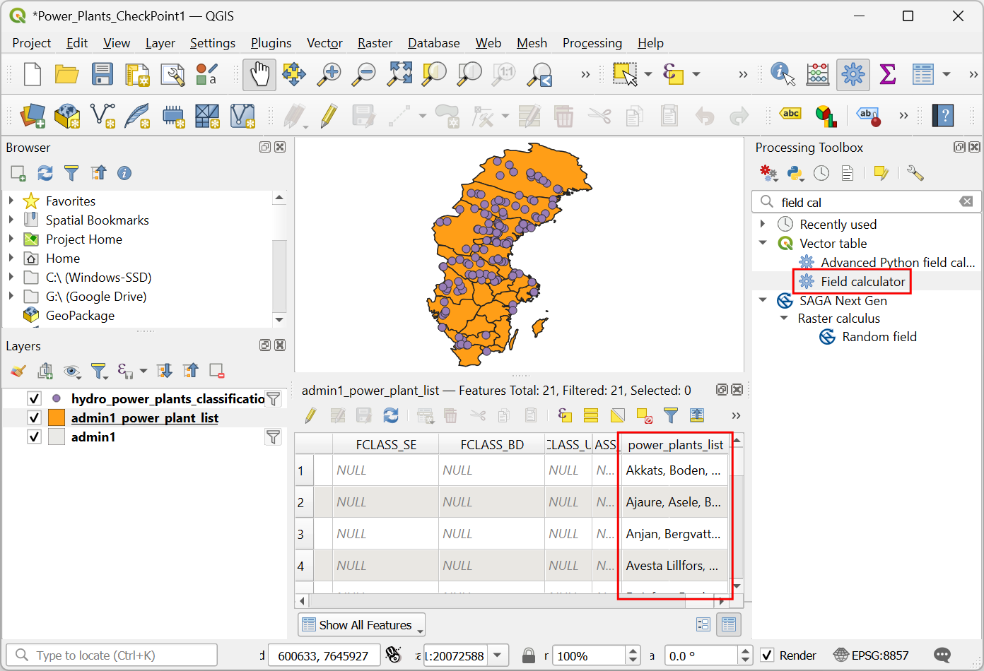
10. Once the processing finishes, a new layer hydro_power_plant_list will be added to the Layers panel. Open the attribute table and verify that the power_plants_list has the list of intersecting power plant names. Next, we will add another column with the total capacity for each region. Open the Vector table → Field calculator algorithm from the Processing Toolbox.

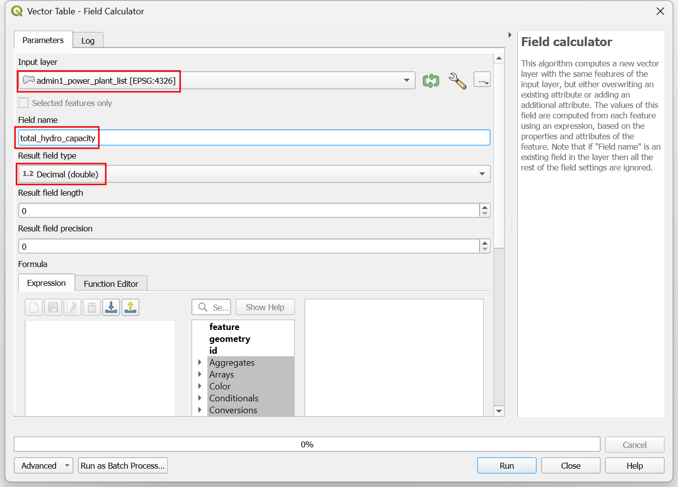
11. In the Vector Table - Field Calculator dialog, select admin1_power_plant_list as the Input Layer. Enter total_hydro_capacity as the Field name. Select Decimal (double) as the Result field type.

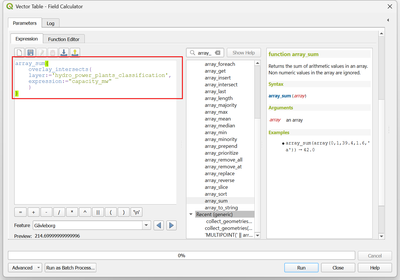
12. Similar to the previous step, we can use the overlay_intersects() function to get a list of values for the capacity_mw attribute for all intersecting power plant features. As we want to calculate the total capacity, we can use the array_sum() function to calculate the total. Enter the following expression.

array_sum(
  overlay_intersects(
    layer:='hydro_power_plants_classification',
    expression:="capacity_mw"
  )
)

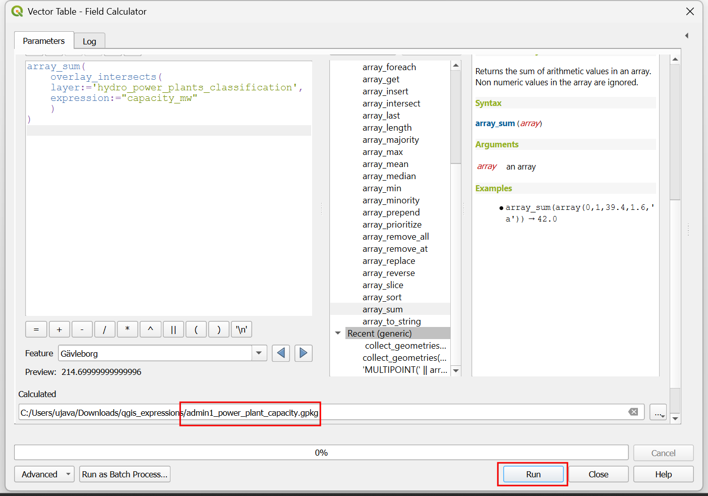
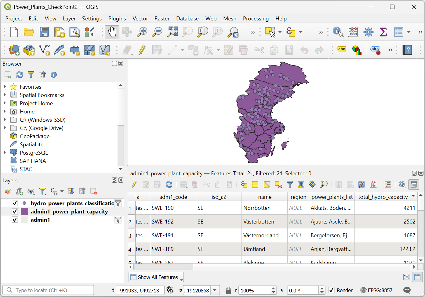
13. Click the … next to Calculated and select Save to File…. Enter the name of the output file as hydro_power_plant_capacity.gpkg and click Run.

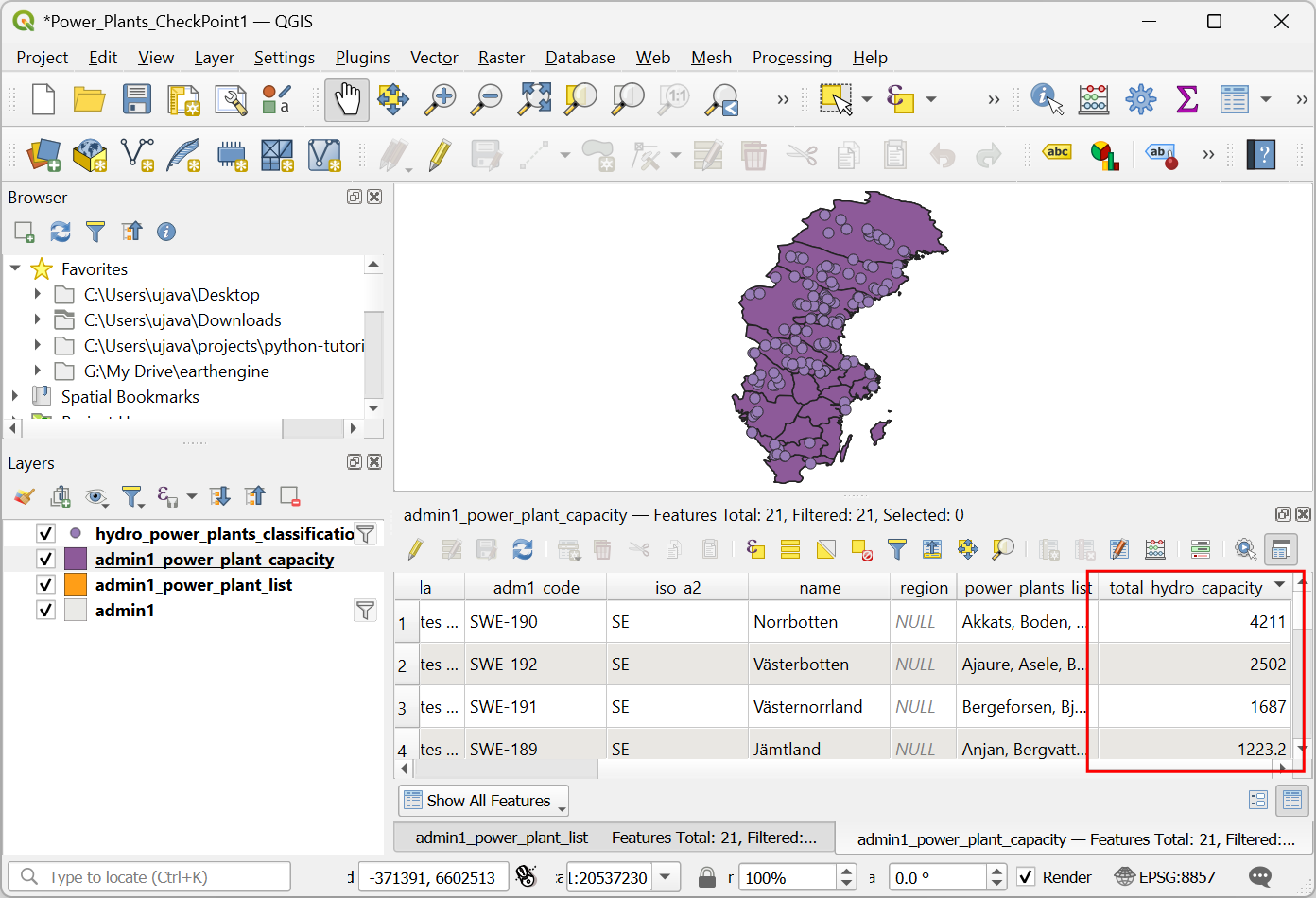
14. Once the processing finishes, a new layer hydro_power_plant_capacity will be added to the Layers panel. Open the attribute table and you will notice that the total_hydro_capacity has the sum of the capacities of all hydro power plants within each region.

15. We are done with the analysis, but often times it i desirable to share the results with others in a non-spatial format. We will not clean up our output and save the data as a spreadsheet. Search and locate the Vector table → Refactor fields algorithm and double-click to launch it.

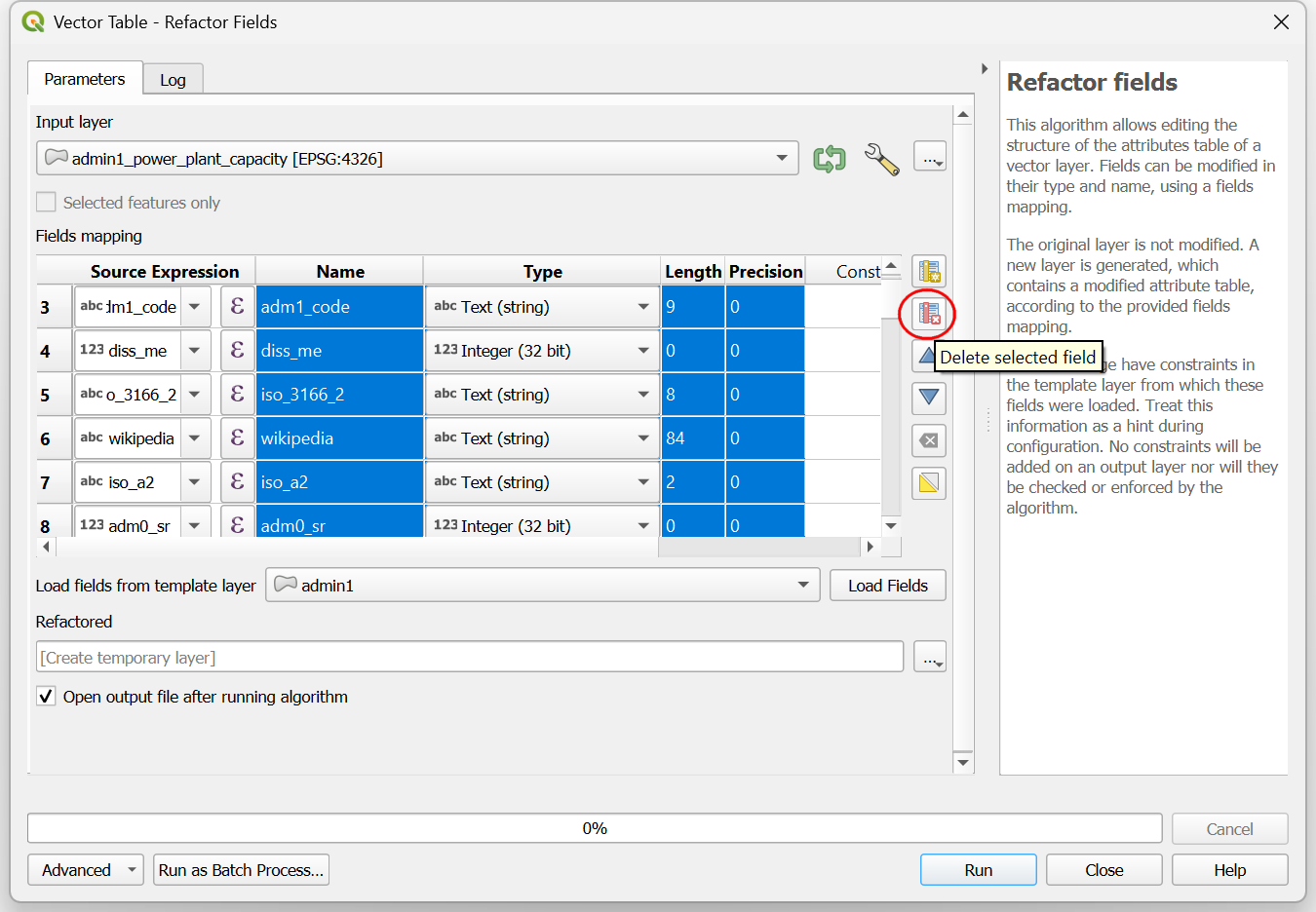
16. Our attribute table contains over 100 columns. We can delete most of them and only keep a few columns in the output. In the Fields mapping section, hold the Shift key and click on the row numbers to select them. Once selected, click the Delete selected field button to remove it from the output.

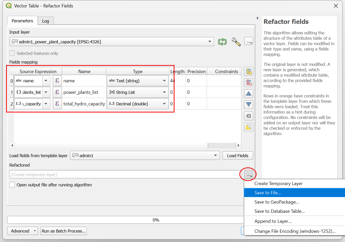
17. For the final output, only keep the name, power_plants_list and total_hydro_capacity fields. Click the … next to Refactored and select Save to File….

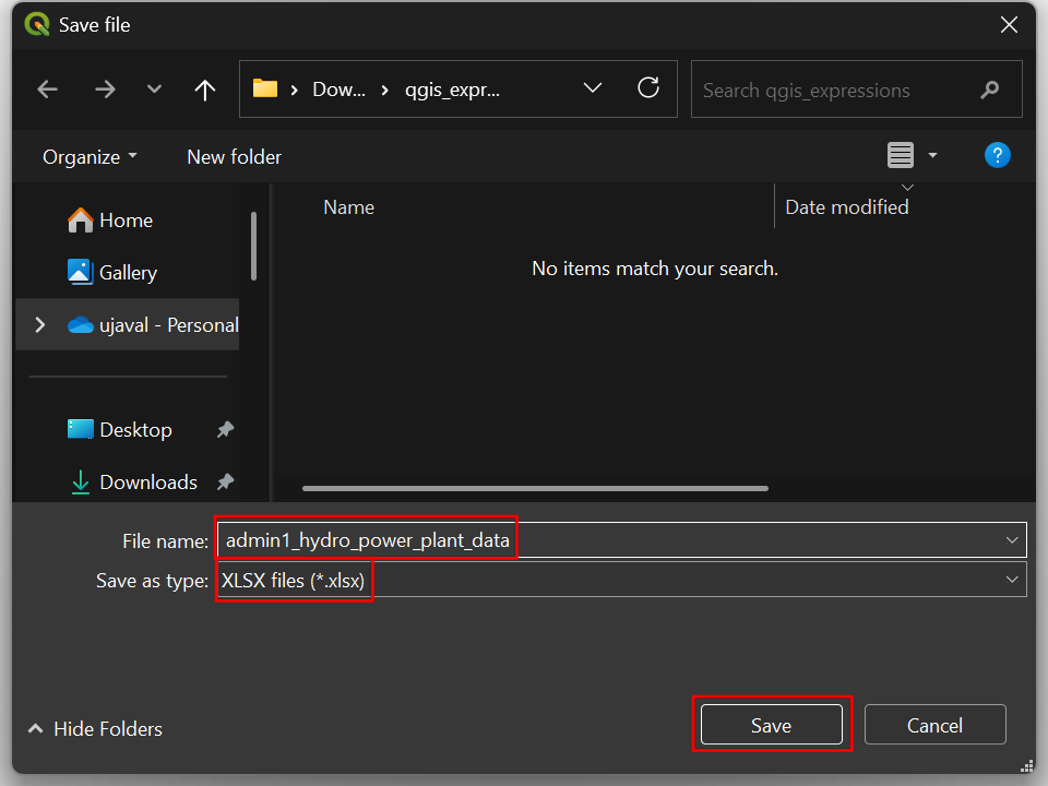
18. In the Save file dialog, choose **XLSX files (*.xlsx)** as the Save as type. Enter the name of the output file as admin1_hydro_power_plant_data and click Save.

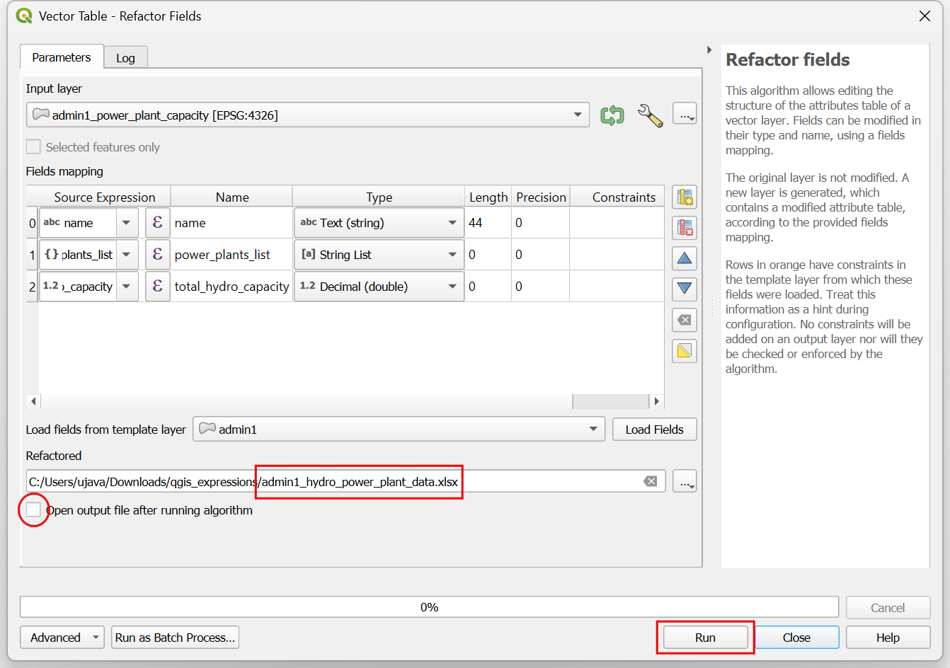
19. Un-check the Open output file after running algorithm box and click Run.

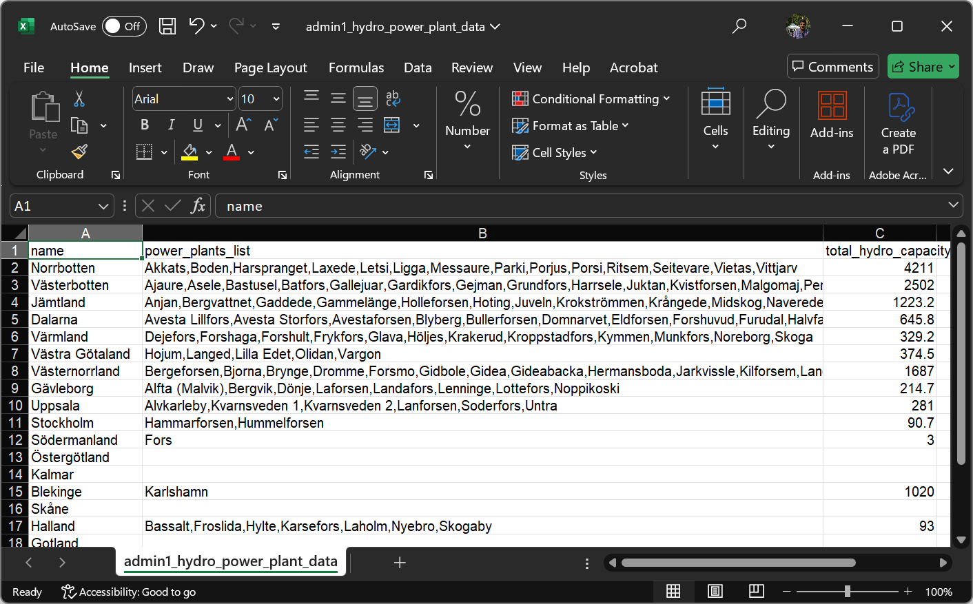
20. Once the processing finishes, open the resulting spreadsheet in Excel or Open Office Calc to see the output.

21. Back in QGIS, we are ready to do the next challenge.

You can load the Power_Plants_CheckPoint2.qgz project in the solutions folder to catch up to this point and do the challenge.

Challenge 2

Add a new column power_plant_count with the total number of hydro power plants in each admin1 region.

Hint: Look under the array_ section to find a suitable function for calculating number of items in a list.

3. Geometries

In this section, we will learn how to create and manipulate feature geometry using expressions. The QGIS expression engine comes with a large number of functions that can be used to create, update, transform geometries of features.

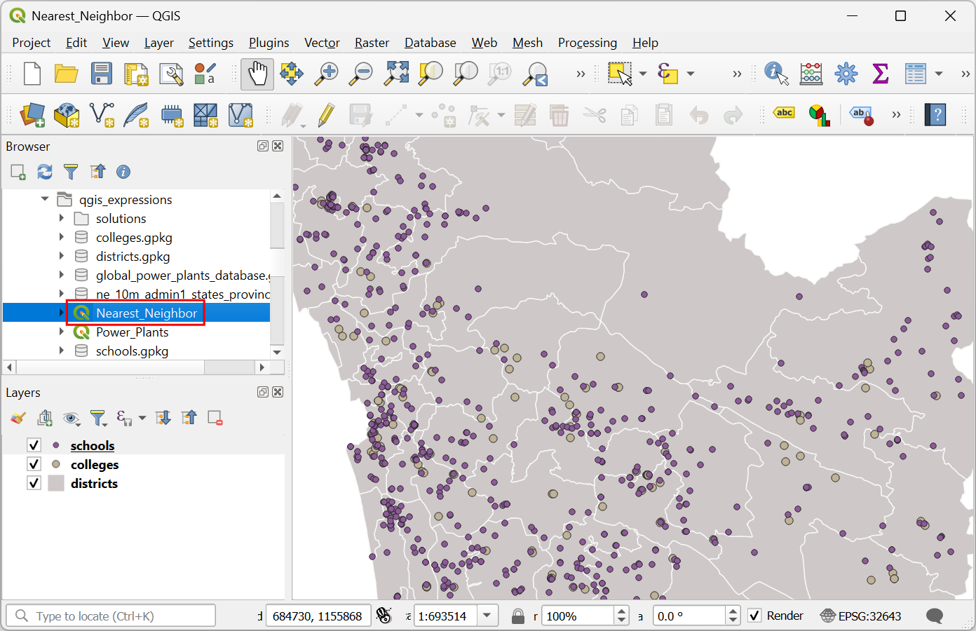
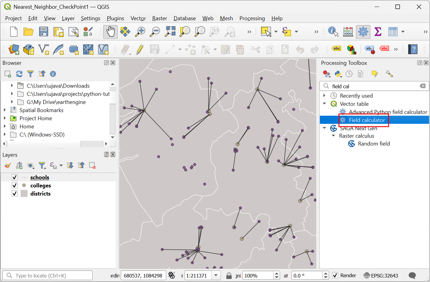
1. Locate and open the Nearest_Neighbor project. This project contains 2 point layers. The layer schools has the locations schools and the layer colleges has locations of all the colleges in the state of Kerala, India. Our goal for this section is to connect each school point to the nearest college point with a line.

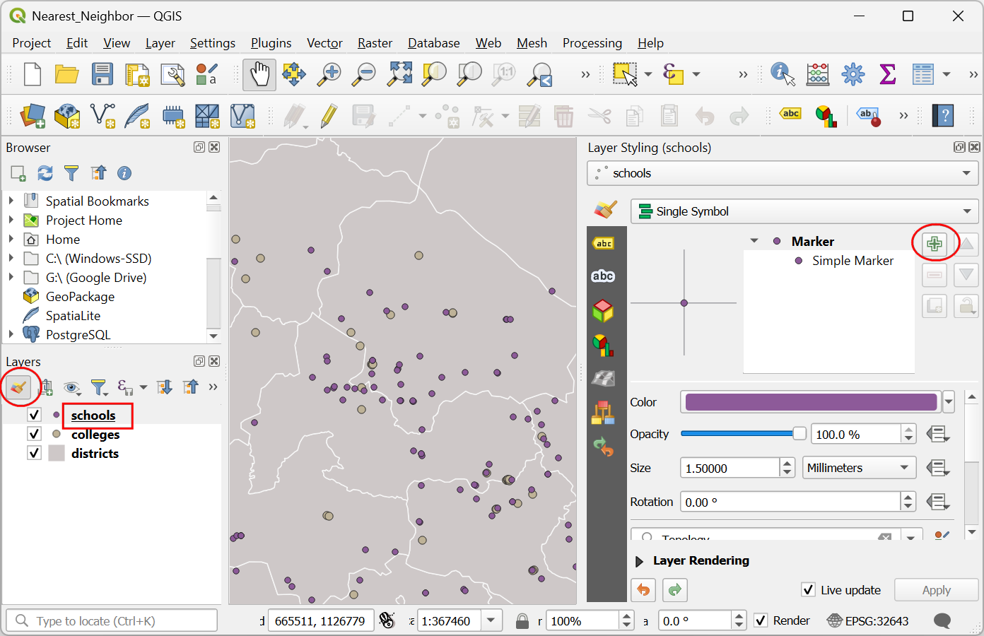
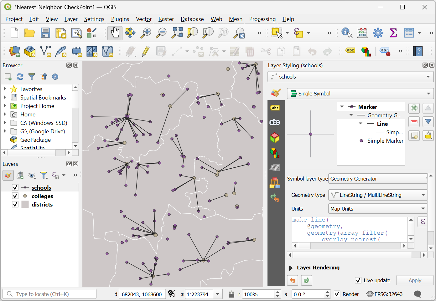
2. Select the schools layer and click the Open the Layer Styling Panel button. The layer is styled using the Simple Marker symbol layer. Click the Add symbol layer / + button.

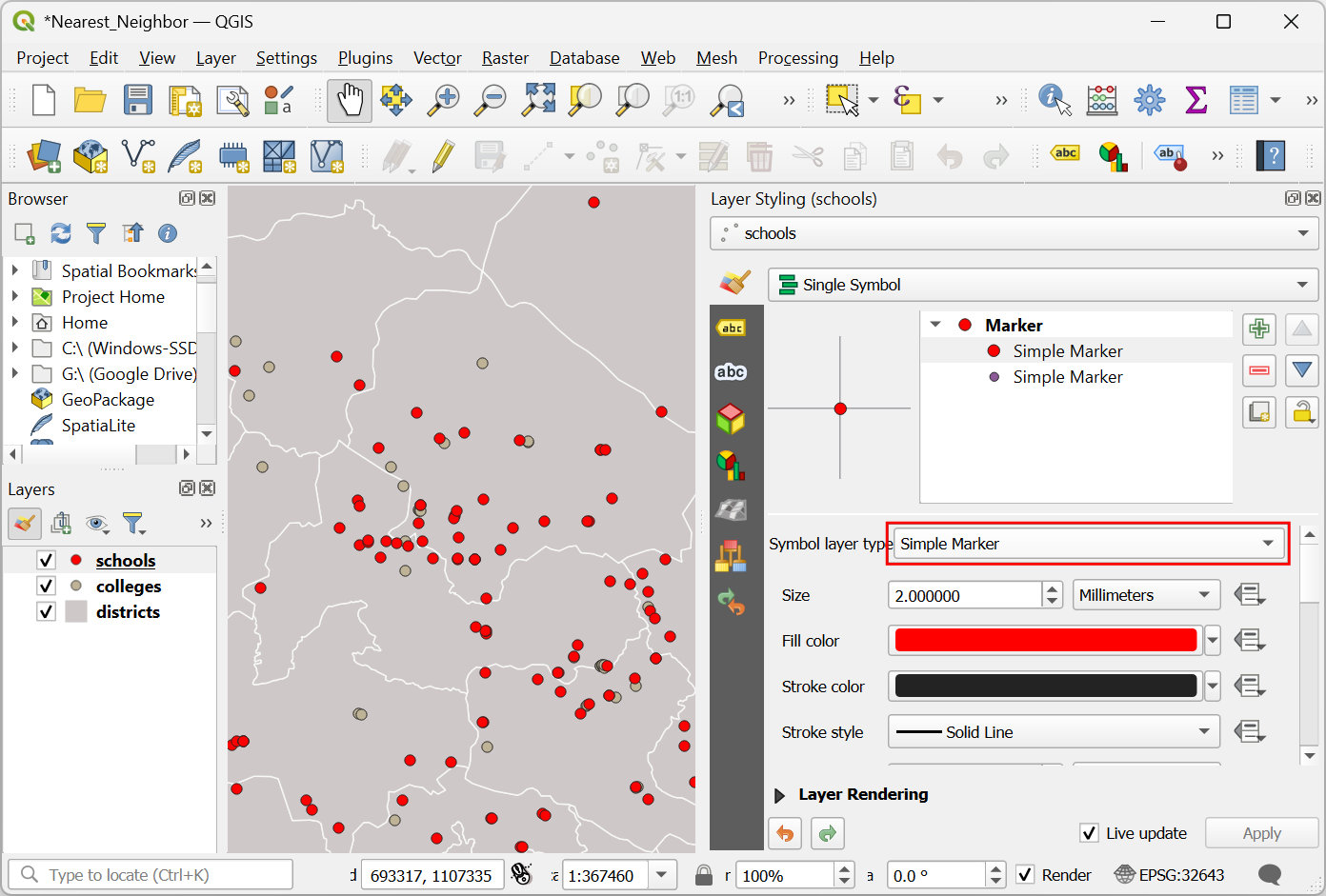
3. A new symbol layer of type Simple Marker will be added. Click on the dropdown next to Symbol layer type and choose Geometry Generator as the Symbol layer type.

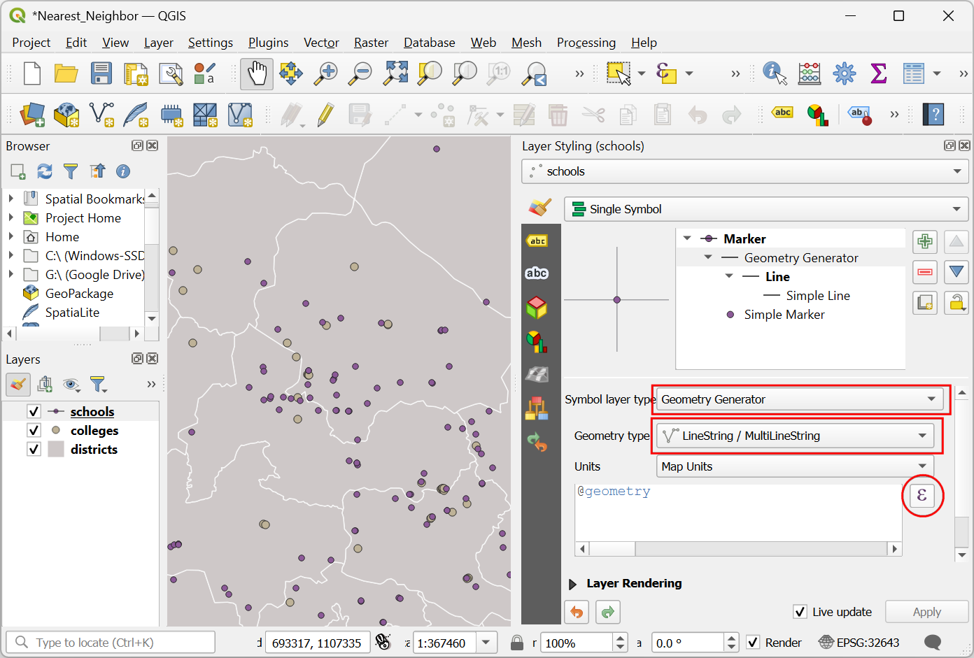
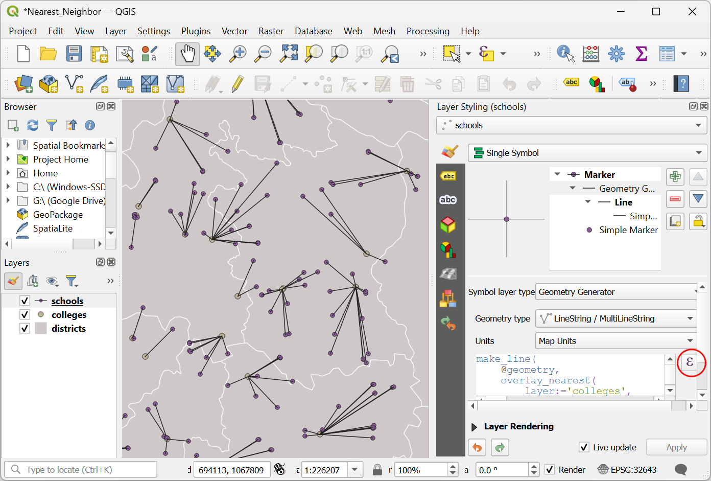
4. Geometry Generator is a special layer type that allows us to write an expression to create new geometries and render them on-the-fly with chosen symbology. As we want to create and render a line, choose LineString / MultiLineString as the Geometry type. Next, click the Expression button.

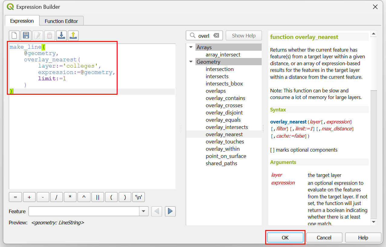
5. We want to find the nearest college to each school feature. The overlay_nearest() function allows us to find nearest features from another layer. We build an expression to find the @geometry of the nearest college and then use the make_line() function to create a line from the school point to the nearest college point. Enter the following expression and click OK.

make_line(
    @geometry,
    overlay_nearest(
        layer:='colleges',
        expression:=@geometry,
        limit:=1
    )
)

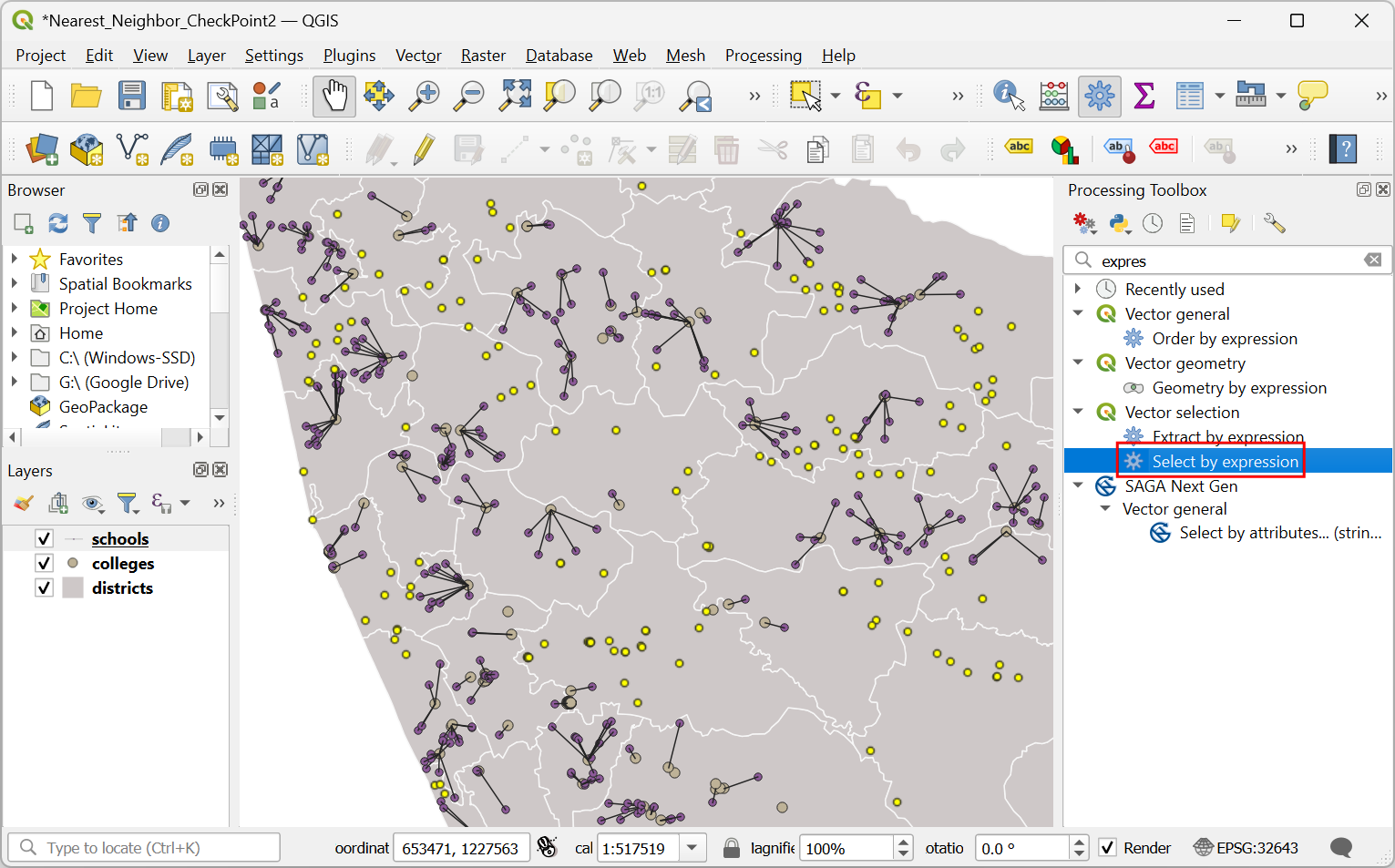
6. You will see the map update and show lines connecting each school feature to the nearest college. These lines are being constructed and rendered on-the-fly using the specified expression. The underlying data-source does not change in any way. Geometry Generator symbol layers are particularly useful for such applications to dynamically visualize the data in a different way. Let’s update the expression. Click the Expression button.

7. The overlay_nearest() function has an optional parameter max_distance that allows us to specify the maximum search distance and only return the feature from another layer within the specified distance. Let’s update the expression to find the nearest college within 5km (5000 meters) distance.

make_line(
    @geometry,
    overlay_nearest(
        layer:='colleges',
        expression:=@geometry,
        limit:=1,
        max_distance:=5000
    )
)

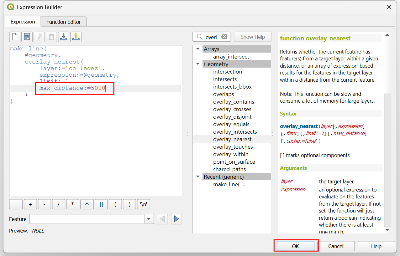
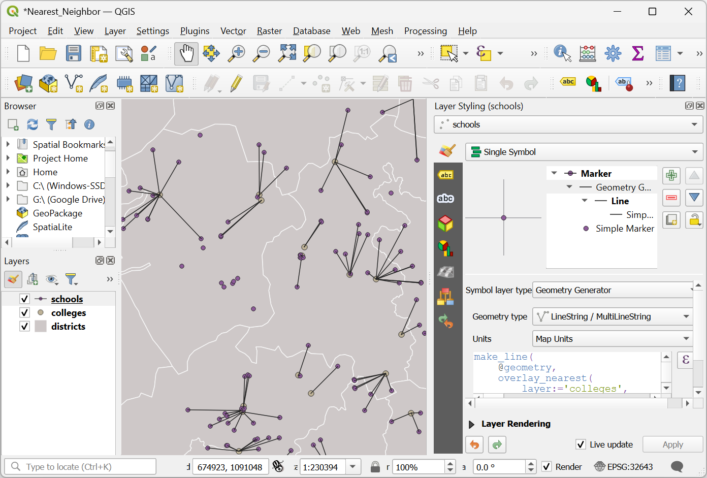
8. The map will update to show the line connections only between schools and colleges within 5km distance.

We have now finished this section. You can load the Nearest_Neighbor_CheckPoint1.qgz project in the solutions folder to catch up to this point and do the challenge.

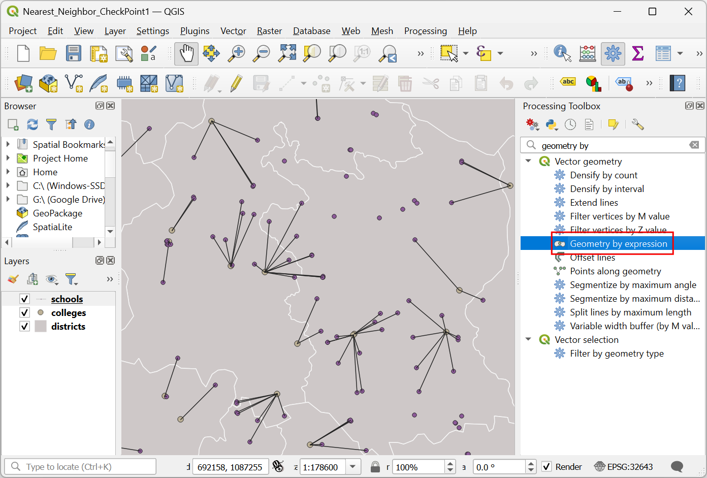
Challenge 3

The Processing Toolbox comes with a handy tool called Geometry by expression. This algorithm allows you to take an input layer and create a new layer by transforming the geometries using expression. Use this tool to create a new layer schools_with_nearest_college.gpkg showing the connections from school points to the nearest college.

4. Iteration

The QGIS expression engine has array functions that allow you to iterate and process each item from the array using expressions. This enables some very powerful use-cases. In this section we will explore the array_foreach() and array_filter() functions.

1. Continuing from the previous section, select the schools layer and open the Vector table → Field calculator algorithm from the Processing Toolbox.

2. In the Vector Table - Field Calculator dialog, select schools as the Input Layer. Enter colleges as the Field name. Select String List as the Result field type.

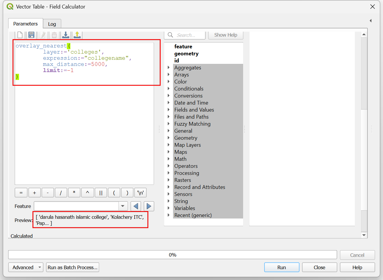
3. We want to get the list of college names within 5km of each school. Enter the following expression and see the output shown in the Preview.

overlay_nearest(
    layer:='colleges',
    expression:="collegename",
    max_distance:=5000,
    limit:=-1
)

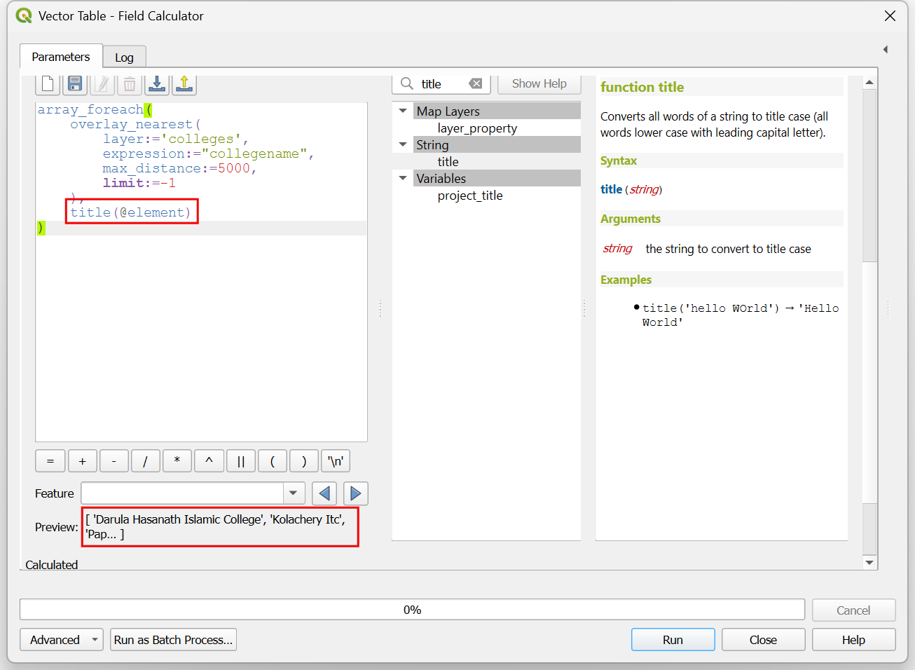
4. Let’s say we want to convert each name to title case. We can use the array_foreach() function which allows us to run an expression on each item. Within the function, you refer to each item in the array with the variable @element. Update the expression as below.

array_foreach(
    overlay_nearest(
        layer:='colleges',
        expression:="collegename",
        max_distance:=5000,
        limit:=-1
    ),
    title(@element)
)

5. Click the … next to Calculated and select Save to File…. Enter the name of the output file as nearest_colleges.gpkg and click Run.

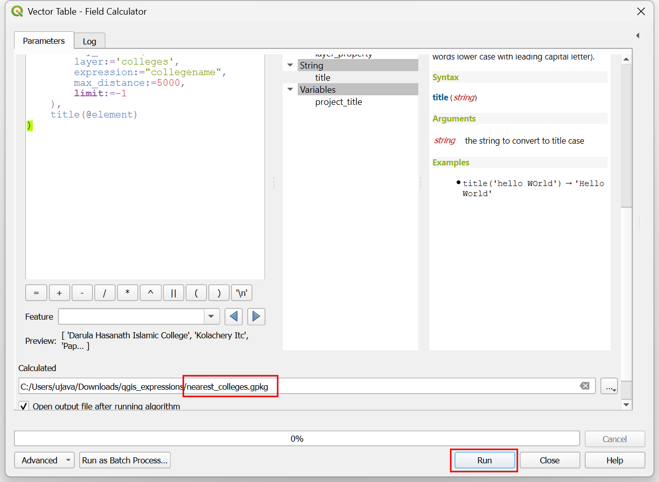
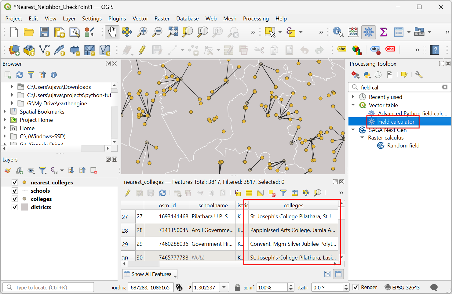
6. Once the processing finishes, a new layer nearest_colleges will be added to the Layers panel. Open the attribute table and you will notice that the colleges column has the list of colleges in title case. Open the Vector table → Field calculator algorithm again.

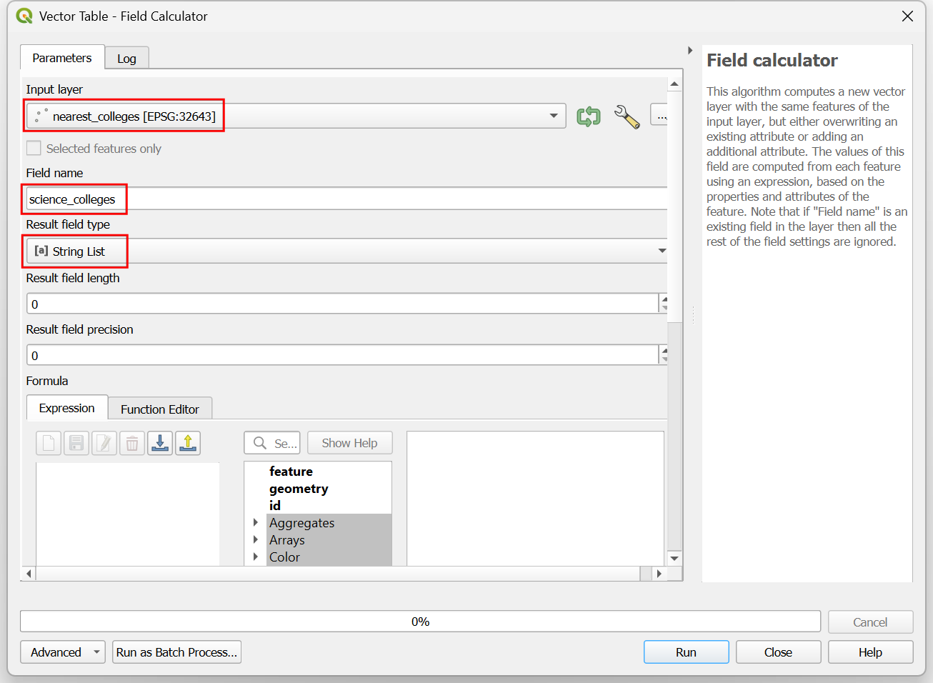
7. In the Vector Table - Field Calculator dialog, select nearest_colleges as the Input Layer. Enter science_colleges as the Field name. Select String List as the Result field type.

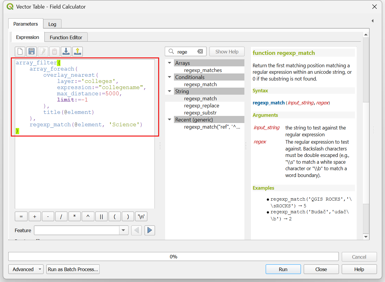
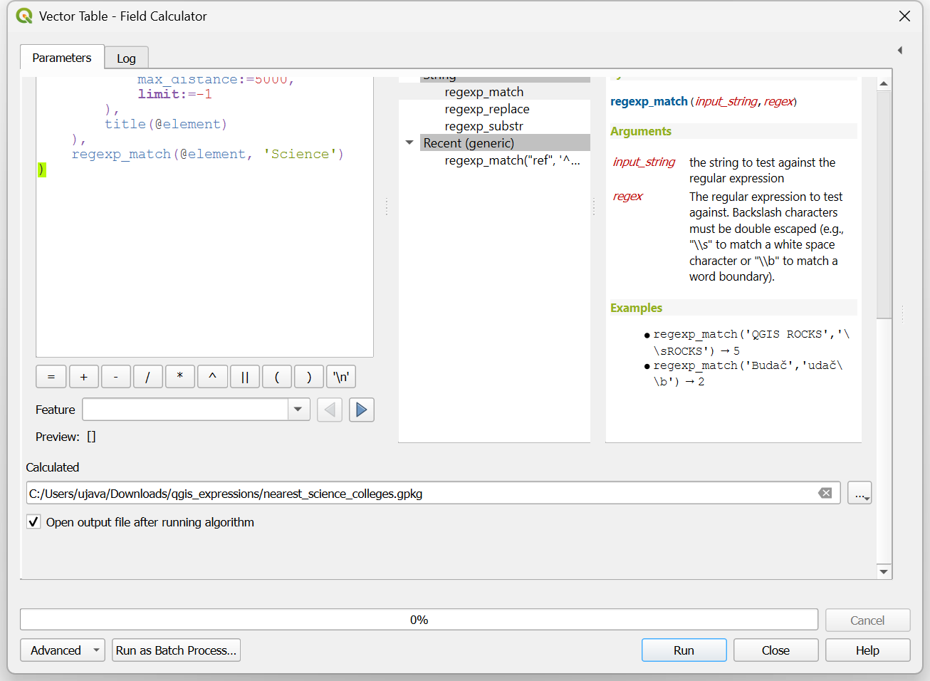
8. From our list of colleges, we want to select only the colleges with the word Science in their names. To achieve this, we can use the array_filter() function to iterate through each item and check if the text is present. This can be achieved using the regexp_match() function. Enter the expression as below.

array_filter(
    array_foreach(
        overlay_nearest(
            layer:='colleges',
            expression:="collegename",
            max_distance:=5000,
            limit:=-1
        ),
        title(@element)
    ),
    regexp_match(@element, 'Science')
)

9. Click the … next to Calculated and select Save to File…. Enter the name of the output file as nearest_science_colleges.gpkg and click Run.

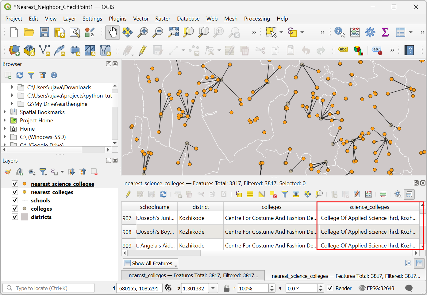
10. Once the processing finishes, a new layer nearest_science_colleges will be added to the Layers panel. Open the attribute table and you will notice that the science_colleges column has the list of colleges containing the keyword Science.

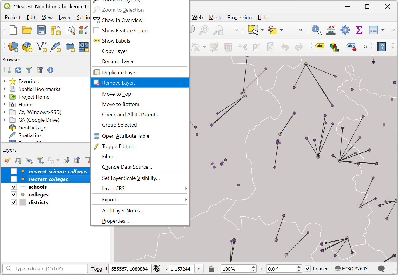
11. Select both the nearest_colleges and nearest_science_colleges layers. Right-click and select Remove Layer.

12. We will now apply these concept of iteration and filtering to our problem of connecting schools to the nearest college. We will apply an additional criteria to connect each school to the nearest college that belongs to the same district as the school. Let’s update the expression to apply this filter. Select the schools layer and click the Open the Layer Styling Panel button. Select the Geometry Generator symbol layer.

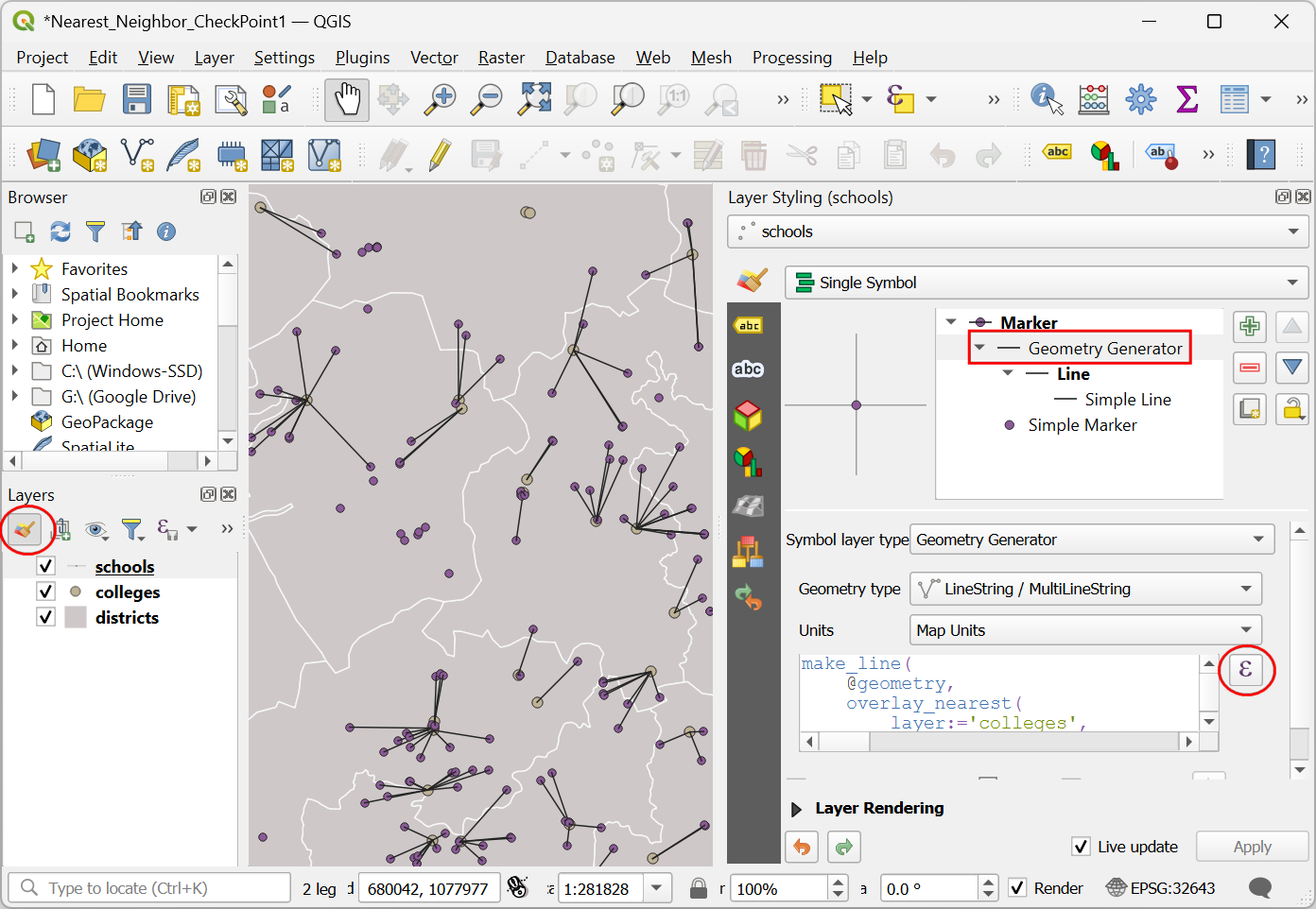
13. We will update the overlay_nearest() function to return us the list of @feature instead of @geometry. This will allow us to run the filter on the attributes. We then use array_filter() to select all college features where the value of district is the same as the value of district for the school. Finally we select the first matching feature using [0] and use geometry() to extract the geometry of the feature. The final expression for creating a line from the school to the nearest college in the same district is as follows.

make_line(
    @geometry,
    geometry(array_filter(
        overlay_nearest(
            layer:='colleges',
            expression:=@feature,
            max_distance:=5000,
            limit:=-1
        ),
    "district"=attribute(@element, 'district'))[0])
)

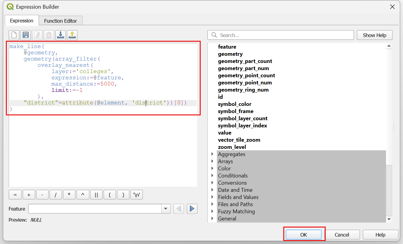
14. Once you apply the expression, the map will update and you will see that each school is now connected to the nearest college that belongs to the same administrative area.

You can now load the Nearest_Neighbor_CheckPoint2.qgz project in the solutions folder to catch up to this point and do the challenge.

Challenge 4

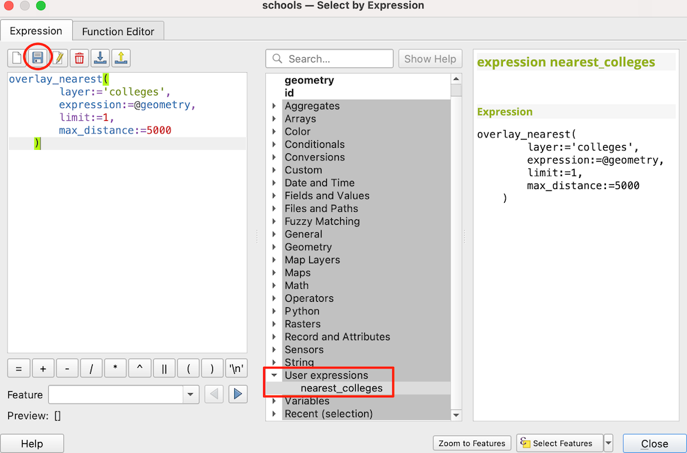
You will notice that there are many schools with no connection to colleges. The challenge is select all schools which have no nearby college in the same district. You can use the Select by expression algorithm in the Processing Toolbox to select features using an expression.

Data Credits

• Admin 1 – States, Provinces: Made with Natural Earth. Free vector and raster map data @ naturalearthdata.com. Admin1 boundaries were edited and combined with countries (India POV) boundaries.
• Global Power Plant Database: Global Energy Observatory, Google, KTH Royal Institute of Technology in Stockholm, Enipedia, World Resources Institute. 2021. Global Power Plant Database version 1.3.0. Accessed through https://datasets.wri.org/datasets/global-power-plant-database on
• School and College locations: Data Copyright 2023 OpenStreetMap Contributors. Downloaded using QuickOSM plugin in QGIS.
• District boundaries: Downloaded from GeoBoundaries. Runfola, D. et al. (2020) geoBoundaries: A global database of political administrative boundaries. PLoS ONE 15(4): e0231866. https://doi.org/10.1371/journal.pone.0231866

License

This workshop material is licensed under a Creative Commons Attribution 4.0 International (CC BY 4.0). You are free to re-use and adapt the material but are required to give appropriate credit to the original author as below:

QGIS Expressions Masterclass by Ujaval Gandhi www.spatialthoughts.com

---

---

If you want to report any issues with this page, please comment below.