Mastering GDAL Tools (Full Course Material)

A practical hands-on introduction to GDAL and OGR command-line programs

---

---

Introduction

GDAL is an open-source library for raster and vector geospatial data formats. The library comes with a vast collection of utility programs that can perform many geoprocessing tasks. This class introduces GDAL and OGR utilities with example workflows for processing raster and vector data. The class also shows how to use these utility programs to build Spatial ETL pipelines and do batch processing.

Watch the Video ↗

Access the Presentation ↗

Setting up the Environment

This course requires installing the GDAL package. Along with GDAL, we highly recommend installing QGIS to view the result of the command-line operations. You will find installation instructions for both the software below.

Install GDAL

The preferred method for installing the GDAL Tools is via Anaconda. Follow these steps to install Anaconda and the GDAL library.

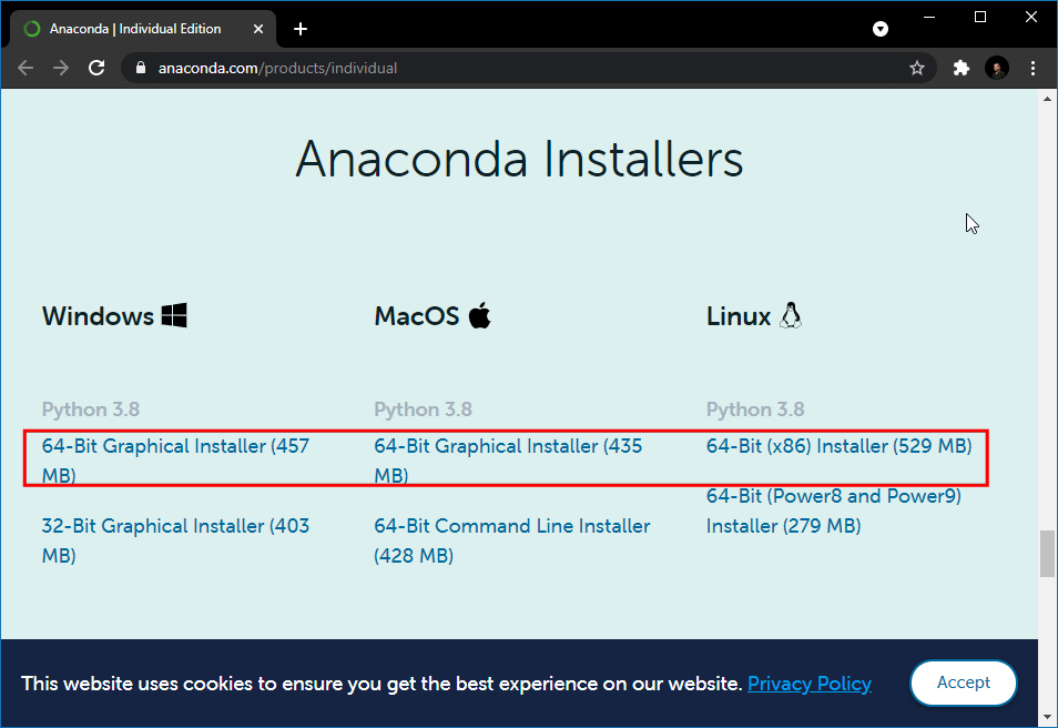
Download the Anaconda Installer for Python 3.7 (or a higher version) for your operating system. Once downloaded, double click the installer and install it into the default suggested directory.

Note: If your username has spaces, or non-English characters, it causes problems. In that case, you can install it to a path such as C:\anaconda.

Windows

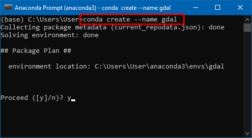
Once Anaconda installed, search for Anaconda Prompt in the Start Menu and launch a new window.

1. Create a new environment named gdal. When prompted to confirm, type y and press Enter.

conda create --name gdal

Note: You can select Right Click → Paste to paste commands in Anaconda Prompt.

2. Activate the environment and install the gdal package. When prompted to confirm, type y and press Enter.

conda activate gdal
conda install -c conda-forge gdal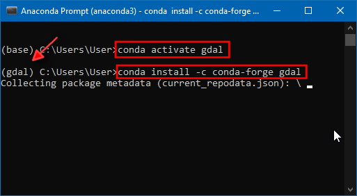

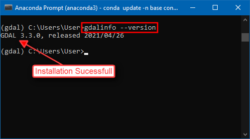
3. Once the installation finishes, verify if you are able to run the GDAL tools. Type the following command and check if a version number is printed.

gdalinfo --version

The version number displayed for you may be slightly different. As long as you do not get a command not found error, you should be set for the class.

Mac/Linux

Once Anaconda is installed, launch a Terminal window.

1. Create a new environment named gdal. When prompted to confirm, type y and press Enter.

conda create --name gdal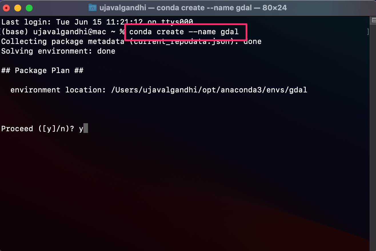

2. Activate the environment and install the gdal package. When prompted to confirm, type y and press Enter.

conda activate gdal
conda install -c conda-forge gdal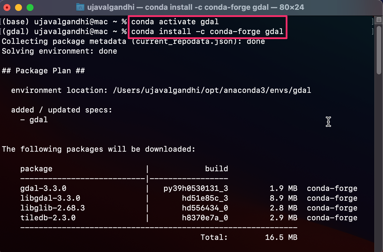

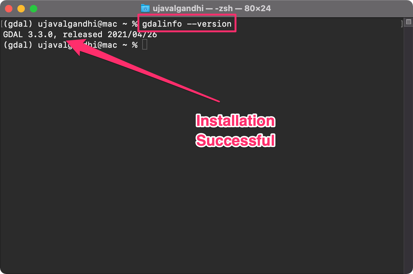
3. Once the installation finishes, verify if you are able to run the GDAL tools. Type the following command and check if a version number is printed.

gdalinfo --version

The version number displayed for you may be slightly different. As long as you do not get a command not found error, you should be set for the class.

Google Colab Notebook [Optional]

We also provide a Google Colab Notebook for the course that allows you to run all the workflows in the cloud without the need to install any packages or download any datasets. You may use this as an alternative environment if you cannot install the software on your machine due to security restrictions.

Install QGIS

This course uses QGIS LTR version for visualization of results. It is not mandatory to install QGIS, but highly recommended.

Please review QGIS-LTR Installation Guide for step-by-step instructions.

Download the Data Package

The code examples in this class use a variety of datasets. All the required datasets are supplied to you in the gdal_tools.zip file. Unzip this file to the Downloads directory. All commands below assume the data is available in the <home folder>/Downloads/gdal_tools/ directory.

Download gdal-tools.zip.

Note: Certification and Support are only available for participants in our paid instructor-led classes.

Get the Course Videos

The course is accompanied by a set of videos covering the all the modules. These videos are recorded from our live instructor-led classes and are edited to make them easier to consume for self-study. We have 2 versions of the videos:

YouTube

We have created a YouTube Playlist with separate videos for each section and exercise to enable effective online-learning. Access the YouTube Playlist ↗

Vimeo

We are also making combined full-length video for each module available on Vimeo. These videos can be downloaded for offline learning. Access the Vimeo Playlist ↗

Getting Familiar with the Command Prompt

All the commands in the exercises below are expected to be run from the Anaconda Prompt on Windows or a Terminal on Mac/Linux. We will now cover basic terminal commands that will help you get comfortable with the environment

Windows

Command	Description	Example
cd	Change directory	cd Downloads\gdal-tools
cd ..	Change to the parent directory	cd ..
dir	List files in the current directory	dir
del	Delete a file	del test.txt
rmdir	Delete a directory	rmdir /s test
mkdir	Create a directory	mkdir test
type	Print the contents of a file	type test.txt
> output.txt	Redirect the output to a file	dir /b > test.txt
cls	Clear screen	cls

Mac/Linux

Command	Description	Example
cd	Change directory	cd Downloads/gdal-tools
cd ..	Change to the parent directory	cd ..
ls	List files in the current directory	ls
rm	Delete a file	rm test.txt
rm -R	Delete a directory	rm -R test
mkdir	Create a directory	mkdir test
cat	Print the contents of a file	cat test.txt
> output.txt	Redirect the output to a file	ls > test.txt
clear	Clear screen	clear

1. GDAL Tools

Start Module Videos ↗

1.1 Basic Raster Processing

We will start learning the basic GDAL commands by processing elevation rasters from SRTM. In the Command Prompt window, use the cd command to change to the srtm directory which 4 individual SRTM tiles around the Mt. Everest region.

cd srtm

Use the gdalinfo command to check the information about a single image.

gdalinfo N28E086.hgt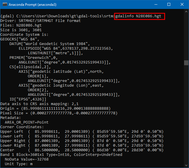

A useful parameter is -stats which computes and displays image statistics. Run it on the raster to get some statistics of pixel values in the image.

gdalinfo -stats N28E086.hgt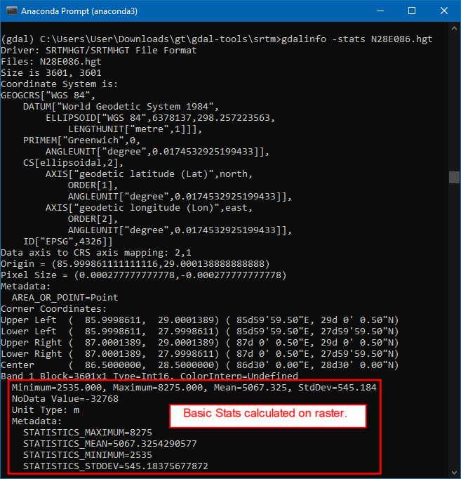

1.1.1 Merging Tiles

We will now merge the 4 neighboring SRTM tiles into 1 raster so we can work with them together. GDAL provides a useful format called Virtual Raster that allows us to create a Virtual file with .vrt extension that is a pointer to multiple source files. A .vrt file is just a text file, so it doesn’t consume any disk space but allows us to run any GDAL command as if it was a raster file.

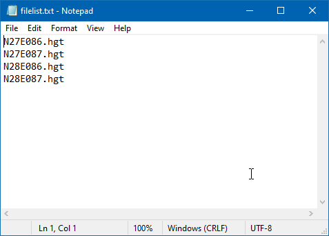
First we need to create a text file containing all the files we want to merge. We can use the dir command on Command prompt to list the files matching the pattern *.hgt and redirect the output to a file. Here the /b option runs the command in the Bare mode which excludes all info except file names.

Windows

dir /b *.hgt > filelist.txt

For Mac/Linux systems, the same can be achieved using the ls command.

Mac/Linux

ls *.hgt > filelist.txt

Once the command finishes, verify that the filelist.txt has the names of the source tiles.

We can now use the gdalbuildvrt program to create a virtual raster from the source files in the filelist.txt.

gdalbuildvrt -input_file_list filelist.txt merged.vrt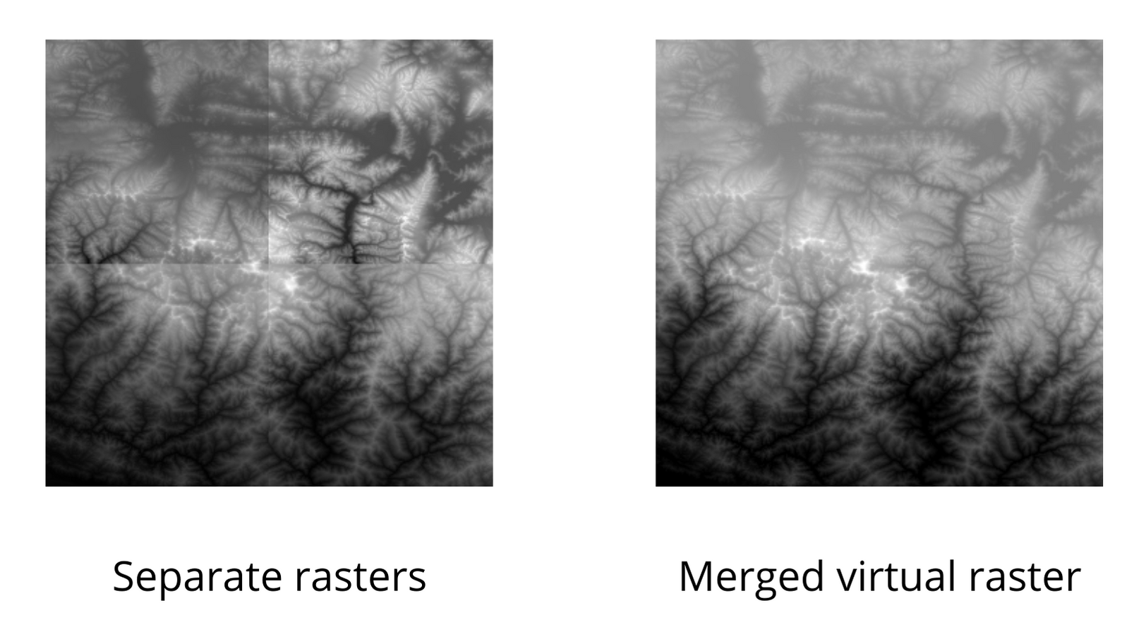

Note: We could have done this operation in a single step using the command gdalbuildvrt merged.vrt *.hgt. However, some versions of GDAL on Windows do not expand the * wildcard correctly and the command results in an error. It is recommended to use a file list instead of wildcards with GDAL commands on Windows to avoid unexpected results.[reference]

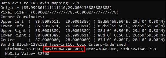
Exercise 1

Can you find what is the highest elevation value in the merged raster? Since these rasters are around the Mt.Everest region, the MAXIMUM value will be the elevation of the summit.

1.1.2 Converting Formats

Let’s convert the Virtual Raster to a GeoTIFF file. gdal_translate program allows us to convert between any of the hundreds of data formats supported by GDAL. The format is recognized from the file extension. Alternatively, you can also specify it using the -of option with the short name of the format such a GTiff.

gdal_translate -of GTiff merged.vrt merged.tif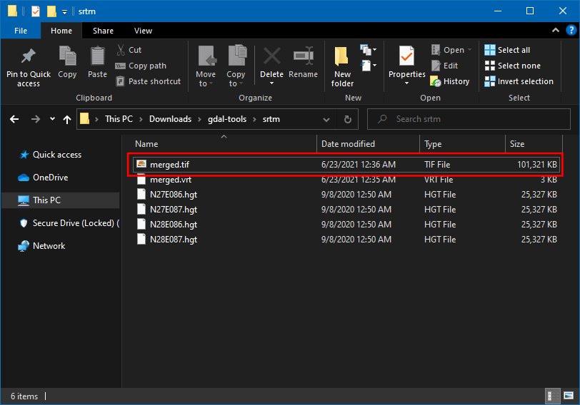

1.1.3 Compressing Output

The default output GeoTIFF file is uncompressed - meaning each pixel’s value is stored on the disk without any further processing. For large rasters, this can consume a lot of disk space. A smart approach is to use a lossless compression algorithm to reduce the size of the raster while maintaining full fidelity of the original data. GDAL supports many compression algorithms out-of-the-box and can be specified with GDAL commands using the -co option. The most popular loss-less compression algorithms are DEFLATE, LZW and PACKBITS. We can try the DEFLATE algorithm on our dataset.

gdal_translate -of GTiff merged.vrt merged.tif -co COMPRESS=DEFLATE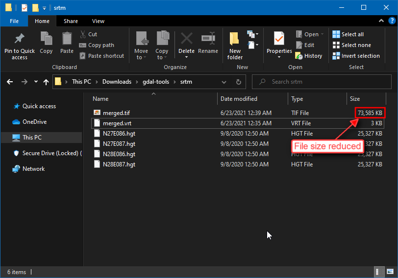

The uncompressed file size was 100+ MB. After applying the DEFLATE compression, the file size was reduced to 75MB. We can further reduce the file size by specifying additional options. The PREDICTOR option helps compress data better when the neighboring values are correlated. For elevation data, this is definitely the case. The TILED option will compress the data in blocks rather than line-by-line.

Note: You can split long commands into multiple lines using the line-continuation character. Windows shell uses ^ as the line-continuation, while Mac/Linux shells use \ as the line continuation.

Windows

gdal_translate -of GTiff merged.vrt merged.tif ^
  -co COMPRESS=DEFLATE -co TILED=YES -co PREDICTOR=2

Mac/Linux

gdal_translate -of GTiff merged.vrt merged.tif \
  -co COMPRESS=DEFLATE -co TILED=YES -co PREDICTOR=2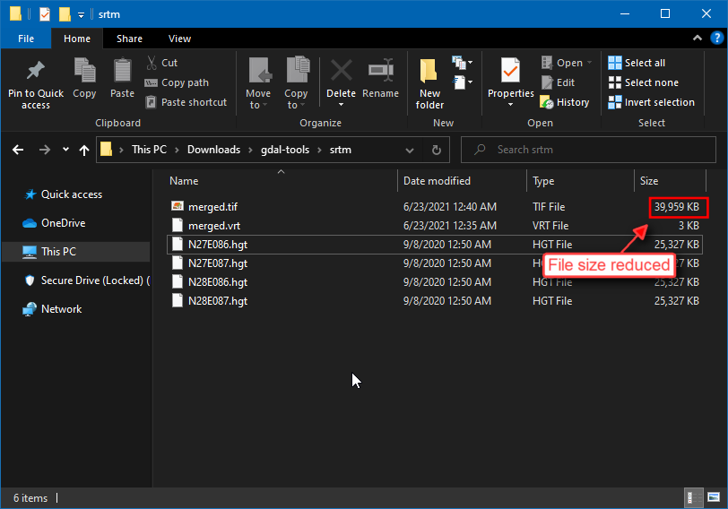

The resulting file now comes out much smaller at 39MB. Check this article GeoTIFF compression and optimization with GDAL to learn more about various options and compression algorithms.

1.1.4 Setting NoData Values

The output from gdalinfo program shows that the original data has a NoData Value set to -32768. We can set a new NoData value. The -a_nodata option allows us to specify a new value.

Windows

gdal_translate -of GTiff merged.vrt merged.tif ^
  -co COMPRESS=DEFLATE -co TILED=YES -co PREDICTOR=2 -a_nodata -9999

Mac/Linux

gdal_translate -of GTiff merged.vrt merged.tif \
  -co COMPRESS=DEFLATE -co TILED=YES -co PREDICTOR=2 -a_nodata -9999

After running the command, you can verify the results using the gdalinfo command.

1.1.5 Writing Cloud-Optimized GeoTIFF (COG)

A new format called Cloud-Optimized GeoTIFF (COG) is making access to such a vast amount of imagery easier to access and analyze. A Cloud-optimized GeoTIFF is behaving just like a regular GeoTIFF imagery, but instead of downloading the entire image locally, you can access portions of imagery hosted on a cloud server streamed to clients like QGIS. This makes it very efficient to access this data and even analyze it - without downloading large files. GDAL makes it very easy to create COG files by specifying the -of COG option. Specifying the -co NUM_THREADS=ALL_CPUS helps speed up the creation process by using all available CPUs for compression and creating internal overviews.

The GDAL COG Driver has the following creation options -co enabled by default.

• Has internal tiling (i.e. -co TILED=YES)
• LZW Compression (i.e. -co COMPRESS=LZW)
• Automatic Selection of Predictor (i.e. -co PREDICTOR=YES chooses appropriate predictor for data type)

Windows

gdal_translate -of COG merged.vrt merged_cog.tif ^
  -co COMPRESS=DEFLATE -co PREDICTOR=YES -co NUM_THREADS=ALL_CPUS ^
  -a_nodata -9999

Mac/Linux

gdal_translate -of COG merged.vrt merged_cog.tif \
  -co COMPRESS=DEFLATE -co PREDICTOR=YES -co NUM_THREADS=ALL_CPUS \
  -a_nodata -9999

1.2 Processing Elevation Data

GDAL comes with the gdaldem utility that provides a suite of tools for visualizing and analyzing Digital Elevation Models (DEM). The tool supports the following modes

• Hillshade
• Slope
• Aspect
• Color-relief
• Terrain Ruggedness Index (TRI)
• Topographic Position Index (TPI)
• Roughness

Am important point to note is that the x, y and z units of the DEM should be of same unit. If you are using data in a Geographic CRS (like EPSG:4326) and the height units are in meters, you must specify a scale value using -s option.

1.2.1 Creating Hillshade

Let’s create a hillshade map from the merged SRTM dataset. The hillshade mode creates an 8-bit raster with a nice shaded relief effect. This dataset has X and Y units in degrees and Z units in meters. So we specify 111120 as the scale value.

gdaldem hillshade merged.tif hillshade.tif -s 111120

gdaldem supports multiple hillshading algorithms. Apart from the default, it currently includes the following algorithms.

• Combined shading (-combined): A combination of slope and oblique shading.
• Multidirectional shading (-multidirectional): A combination of hillshading illuminated from 225 deg, 270 deg, 315 deg, and 360 deg azimuth.

Let’s create a hillshade map with the -multidirectional option.

gdaldem hillshade merged.tif hillshade_combined.tif -s 111120 -multidirectional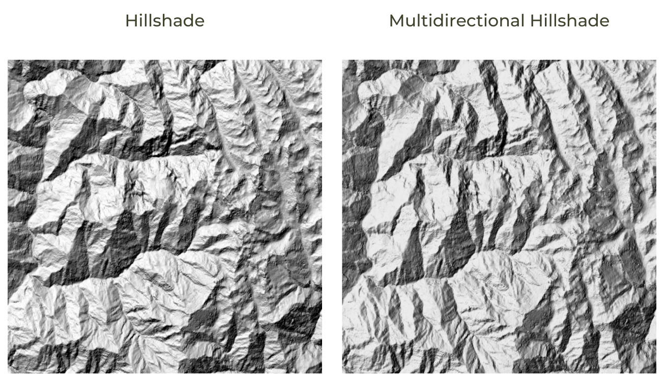

Creating hillshade that is representative of a terrain is more of an ‘art’ than science. The best hand-drawn relief shading is still done manually by cartographers. Recent advances in Deep Learning have shown promise to reproduce the state-of-the-art relief shading using automated techniques. Learn more about Cartographic Relief Shading with Neural Networks and the accompanying software Eduard.

1.2.2 Creating Color Relief

A color relief map is an elevation map where different ranges of elevations are colored differently. The color-relief mode can create a color relief map with the colors and elevation ranges supplied in a text file.

We need to supply the colormap using a text file. Create a new file called colormap.txt with the following content and save it in the same directory as merged.tif. The format of the text file is elevation, red, green, blue values.

1000,101,146,82
1500,190,202,130
2000,241,225,145
2500,244,200,126
3000,197,147,117
4000,204,169,170
5000,251,238,253
6000,255,255,255

We can supply this file to create a colorized elevation map.

gdaldem color-relief merged.tif colormap.txt colorized.tif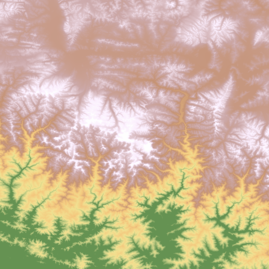

Color Relief

Exercise 2

Save the color relief in the PNG format.

1.3 Processing Aerial Imagery

Use the cd command to change to the naip directory which contains individual aerial imagery tiles in the JPEG2000 format.

cd naip

1.3.1 Create a preview image from source tiles

The source imagery is heavily compressed and covers a large region. Instead of loading the full resolution tiles in a viewer, it is a good practice to create a preview mosaic that can help us assess the coverage and quality of the data.

We first create a Virtual Raster mosaic from all the .jp2 tiles. We can create a text file containing all the files we want to merge.

Windows

dir /b *.jp2 > filelist.txt

Mac/Linux

ls *.jp2 > filelist.txt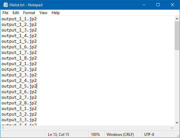

Text File with the List of Images

We are working with Photometric RGB tiles and want to apply JPEG compression on the result. To avoid JPEG artifact and maintain nodata values, it is a good practice to add an Alpha band which will contain the mask containing all valid pixels. We use the -addalpha option to create an alpha band.

gdalbuildvrt -addalpha -input_file_list filelist.txt naip.vrt

We can use the -outsize option and specify a percentage to generate a smaller size preview. The below command generates a 2% preview image in JPEG format. Since we have a 4-band image, we specify which bands to be used for generating the JPG image using the -b option.

gdal_translate -b 1 -b 2 -b 3 -of JPEG -outsize 2% 2% naip.vrt naip_preview.jpg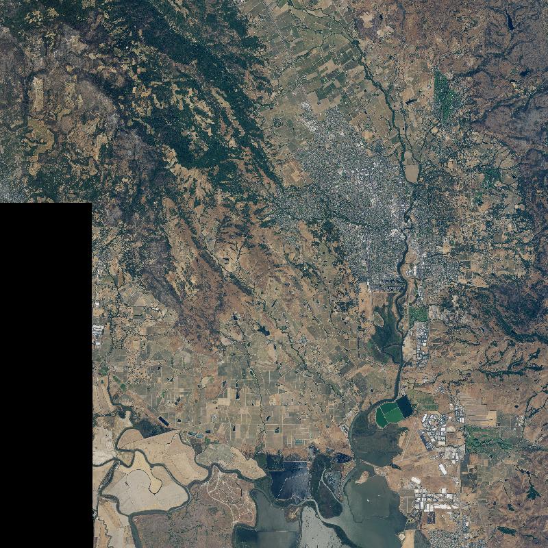 

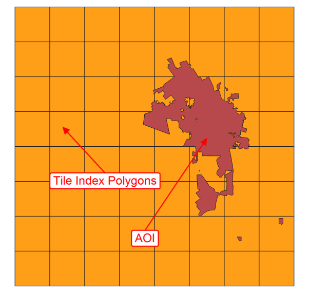
1.3.2 Create a Tile Index

When working with large amounts of imagery tiles, it is useful to generate a tile index. A tile index layer is a polygon layer with the bounding box of each tile. An index layer allows us to check the coverage of the source data and locate specific tiles. It is a simple but effective way to catalog raster data from a hard drive or from a folder on your computer.

gdaltindex program creates a tile index from a list of input files. Here we can use the --optfile option to supply the list of files via a file.

gdaltindex -write_absolute_path index.shp --optfile filelist.txt

1.3.3 Mosaic and clip to AOI

Let’s say we want to mosaic all the source tiles into a single image. We also want to clip the mosaic to a given AOI.

We can use the gdalwarp utility to clip the raster using the -cutline option.

gdalwarp -cutline aoi.shp  -crop_to_cutline naip.vrt aoi_cut.tif -co COMPRESS=DEFLATE -co TILED=YES

We can also add JPEG compression to the output file to reduce the file size. Refer to the post GeoTiff Compression for Dummies by Paul Ramsey that gives more insights into compression imagery. Note that JPEG is a lossy compression method and can cause edge artifacts for image mosaics. To prevent this, we specify the --config GDAL_TIFF_INTERNAL_MASK YES option that uses the mask from the alpha band.

Windows

gdal_translate aoi_cut.tif aoi.tif ^
  -co COMPRESS=JPEG -co TILED=YES -co PHOTOMETRIC=YCBCR -co JPEG_QUALITY=75 ^
  -b 1 -b 2 -b 3 -mask 4 --config GDAL_TIFF_INTERNAL_MASK YES

Mac/Linux

gdal_translate aoi_cut.tif aoi.tif \
  -co COMPRESS=JPEG -co TILED=YES -co PHOTOMETRIC=YCBCR -co JPEG_QUALITY=75 \
  -b 1 -b 2 -b 3 -mask 4 --config GDAL_TIFF_INTERNAL_MASK YES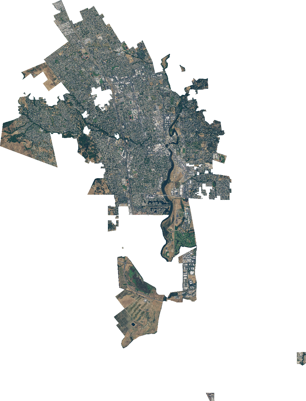

1.3.4 Creating Overviews

If you try loading the resulting raster into a viewer, you will notice that it takes a lot of time for it to render. Zoom/Pan operations are quite slow as well. This is because the viewer is rendering all the pixels at native resolution. Since this is a very high-resolution dataset, it requires processing a lot of pixels, even if you are zoomed out. A common solution to this problem is to create Pyramid Tiles or Overviews. This process creates low-resolution versions of the image by averaging pixel values from higher resolution pixels. If the pyramid tiles are present, imagery viewers can use it to speed up the rendering process. GDAL provides the utility gdaladdo to create overview tiles. GeoTIFF format supports storing the overviews within the file itself. For other formats, the program generates external overviews in the .ovr format.

You can run the gdaladdo (GDAL-Add-Overview) command with default options to create internal overviews. Once the overviews are created, try opening the aoi.tif in QGIS. You will see that it renders much faster and zoom/pan operations are very smooth.

gdaladdo aoi.tif

The default overviews use the nearest neighbor resampling. We can pick any resampling method from the many available algorithms. We can try the bilinear interpolation using the -r bilinear option. Since the source imagery is JPEG compressed, we will compress the overviews with the same compression.

gdaladdo -r bilinear --config COMPRESS_OVERVIEW JPEG aoi.tif

1.4 Processing Satellite Imagery

This section shows how to use the satellite data from Landsat-8 and create various derived products. Use the cd command to switch to the landsat8 directory which contains Landsat-8 imagery. This directory has 5 individual GeoTIFF files for 5 different bands from a single landsat-8 scene.

Band Number	Band Name
B2	Blue
B3	Green
B4	Red
B5	Near Infrared
B8	Panchromatic

cd landsat8

1.4.1 Merging individual bands into RGB composite

Let’s create an RGB composite image by combining three 3 different bands - Red, Green and Blue - into a single image. Here we must use the -separate option which tells the command to place each image in a separate band.

Note: GDAL tools also have a gdal_merge.py script that can also merge rasters into an image. But this script loads all rasters into memory before merging them. This can lead to excessive RAM usage and out of memory errors when working with large files. gdal_merge.py can also be slower than using gdal_translate - when you have large files. So a preferred approach for merging large files would be using the virtual raster as shown here.

Windows

gdalbuildvrt -o rgb.vrt -separate ^
  RT_LC08_L1TP_137042_20190920_20190926_01_T1_2019-09-20_B4.tif ^
  RT_LC08_L1TP_137042_20190920_20190926_01_T1_2019-09-20_B3.tif ^
  RT_LC08_L1TP_137042_20190920_20190926_01_T1_2019-09-20_B2.tif

Mac/Linux

gdalbuildvrt -o rgb.vrt -separate \
  RT_LC08_L1TP_137042_20190920_20190926_01_T1_2019-09-20_B4.tif \
  RT_LC08_L1TP_137042_20190920_20190926_01_T1_2019-09-20_B3.tif \
  RT_LC08_L1TP_137042_20190920_20190926_01_T1_2019-09-20_B2.tif

Then use gdal_translate to merge them.

gdal_translate rgb.vrt rgb.tif -co PHOTOMETRIC=RGB -co COMPRESS=DEFLATE 

Once the command finishes, you can view the result in QGIS.

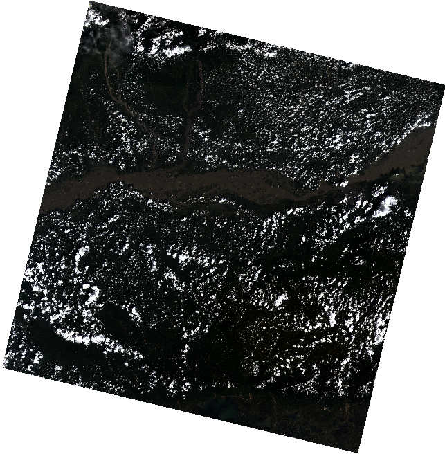
1.4.2 Apply Histogram Stretch and Color Correction

The resulting composite appears quite dark and has low-contrast. QGIS applies a default contrast stretch based on the minimum and maximum values in the image. Due to the presence of clouds and cloud-shadows - there are outlier pixels that make the default contrast stretch not optimal.

Here’s what the histogram of the RGB composite looks like.

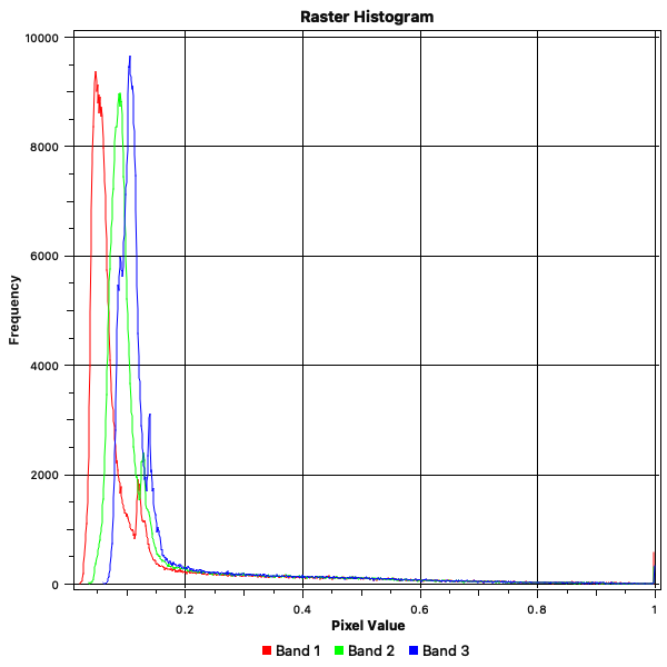
We can apply a histogram stretch to increase the contrast. This is done using the -scale option. Since most of the pixels have a value between 0 and 0.3, we can choose these are minimum and maximum values and apply a contrast stretch to make them go from 0 to 255. The resulting image will be an 8-bit color image where the input pixel values are linearly scaled to the target value.

Note: Scaling the image will alter the pixel values. The resulting image is suitable for visualization, but they should never be used for analysis. Scientific analysis should always use the un-scaled pixel values.

gdal_translate -scale 0 0.3 0 255 -ot Byte rgb.tif rgb_stretch.tif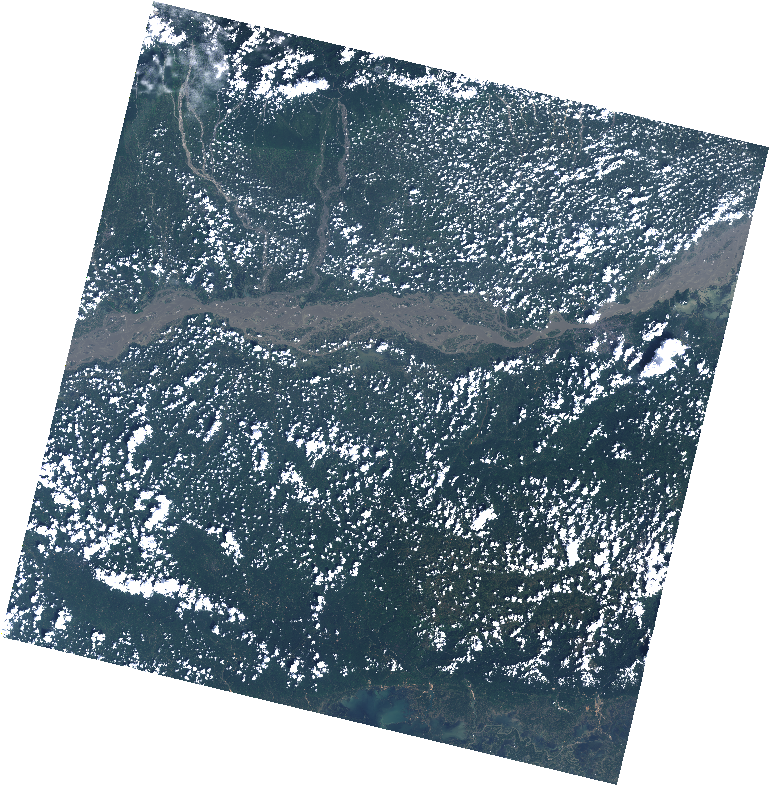

RGB Composite with Linear Stretch

We can also apply a non-linear stretch. gdal_translate has a -exponent option that scales the input values using the following formula. Choosing an exponent value between 0 and 1 will enhance low intensity values - resulting in a brighter image. Learn more

Let’s try exponent value of 0.5. The result is a much better looking output.

gdal_translate -scale 0 0.3 0 255 -exponent 0.5 -ot Byte rgb.tif rgb_stretch.tif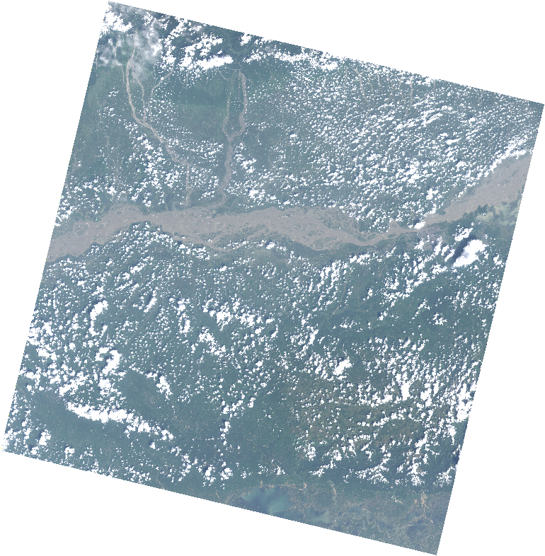

RGB Composite with Exponential Stretch

1.4.3 Raster Algebra

For raster algebra operations, GDAL provides a raster calculator program gdal_calc.py. The input rasters are specified using any letters from A-Z. These letters can be then referenced in the expression. The expression is specified using the --calc option and it supports NumPy syntax and functions.

gdalinfo -stats RT_LC08_L1TP_137042_20190920_20190926_01_T1_2019-09-20_B4.tif

It is important to set NoData value. As seen from the output above, NoData is set to -999.

Note that Windows users need to specify the full path to the GDAL scripts and run it with the python command as shown below. Mac/Linux users can just type the script name directly but if you get an error, you can also specify the full path on Mac/Linux as python $CONDA_PREFIX/bin/gdal_merge.py

Windows

python %CONDA_PREFIX%\Scripts\gdal_calc.py ^
  -A RT_LC08_L1TP_137042_20190920_20190926_01_T1_2019-09-20_B5.tif ^
  -B RT_LC08_L1TP_137042_20190920_20190926_01_T1_2019-09-20_B4.tif ^
  --outfile ndvi.tif --calc="(A-B)/(A+B)" --NoDataValue=-999

Mac/Linux

gdal_calc.py -A RT_LC08_L1TP_137042_20190920_20190926_01_T1_2019-09-20_B5.tif \
  -B RT_LC08_L1TP_137042_20190920_20190926_01_T1_2019-09-20_B4.tif \
  --outfile ndvi.tif --calc="(A-B)/(A+B)" --NoDataValue=-999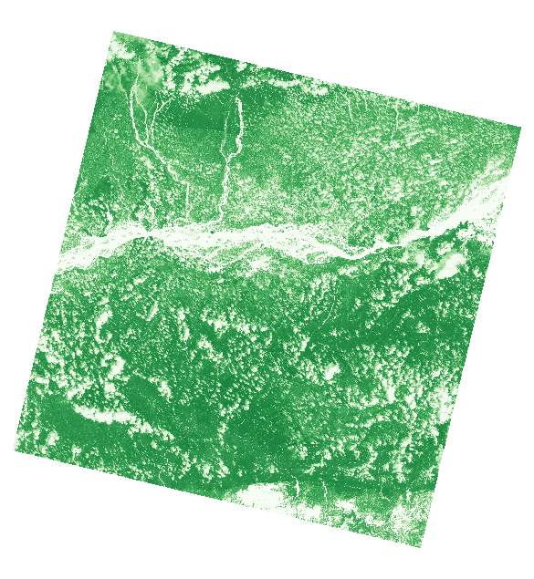

Exercise 3

Create an NRG Composite image with Near Infrared, Red and Green bands. Apply a contrast stretch to the result and save it as a PNG image.

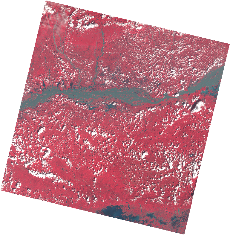
NRG Composite

1.4.4 Pan Sharpening

Most satellite and airborne sensors capture images in the Pan-chromatic band along with other spectral bands. The Red, Green, and Blue bands capture signals in the Red, Green, and Blue portions of the electromagnetic spectrum respectively. But the Pan-band captures the data across the entire range of wavelengths in the visible spectrum. This allows the sensor to capture the data in a higher spatial resolution than other bands which capture the signal from a subset of this wavelength range.

Landsat-8 satellite produces images at a 30m spatial resolution in the Red, Green, Blue bands and at a 15m spatial resolution in the Panchromatic band. We can use the higher spatial resolution of the Panchromatic band to improve the resolution of the other bands, resulting in a sharper image with more details. This process is called Pan-Sharpening.

GDAL comes with a script gdal_pansharpen.py that implements the Brovey algorithm to compute the pansharpened output. In the example below we fuse the 15m resolution panchromatic band (B8) with the RGB composite created in the previous step.

Windows

python %CONDA_PREFIX%\Scripts\gdal_pansharpen.py RT_LC08_L1TP_137042_20190920_20190926_01_T1_2019-09-20_B8.tif ^
  rgb.tif pansharpened.tif -r bilinear -co COMPRESS=DEFLATE -co PHOTOMETRIC=RGB

Mac/Linux

gdal_pansharpen.py RT_LC08_L1TP_137042_20190920_20190926_01_T1_2019-09-20_B8.tif \
  rgb.tif pansharpened.tif -r bilinear -co COMPRESS=DEFLATE -co PHOTOMETRIC=RGB

We can apply the same contrast stretch as before and compare the output. You will notice that the resulting composite is much sharper and can resolve the details in the scene much better.

Windows

gdal_translate -scale 0 0.3 0 255 -exponent 0.5 -ot Byte -a_nodata 0 ^
  pansharpened.tif pansharpened_stretch.tif

Mac/Linux

gdal_translate -scale 0 0.3 0 255 -exponent 0.5 -ot Byte -a_nodata 0 \
  pansharpened.tif pansharpened_stretch.tif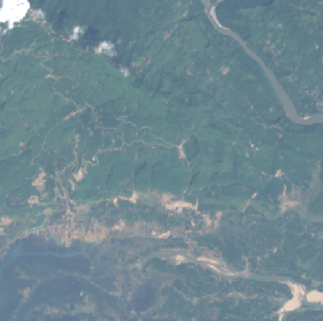

1.5 Processing WMS Layers

GDAL supports reading from a variety of web services, including Web Map Services (WMS) layers.

1.5.1 Listing WMS Layers

NASA’s Socioeconomic Data and Applications Center (SEDAC) provides many useful data layers though WMS Services. We can pick the URL for the appropriate service and list all available layers using gdalinfo.

gdalinfo "WMS:https://sedac.ciesin.columbia.edu/geoserver/ows?version=1.3.0"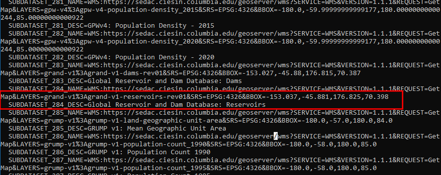

We can get more information about a particular layer by specifying the output from the command above. Let’s get more info about the Global Reservoir and Dam (GRanD), v1 layer.

gdalinfo "WMS:https://sedac.ciesin.columbia.edu/geoserver/ows?SERVICE=WMS&VERSION=1.3.0&REQUEST=GetMap&LAYERS=grand-v1%3Agrand-v1-reservoirs-rev01&CRS=CRS:84&BBOX=-153.037,-45.881,176.825,70.398"

1.5.2 Creating a Service Description File

GDAL can also create a Service Description XML file from a WMS layer. Many GIS programs, including QGIS recognize these XML files as valid raster layers. This allows users to easily drag-and-drop them into their favorite viewer to access a WMS service without any configuration. gdal_translate can write the WMS XML files by specifying -of WMS option.

gdal_translate -of WMS "WMS:https://sedac.ciesin.columbia.edu/geoserver/ows?SERVICE=WMS&VERSION=1.3.0&REQUEST=GetMap&LAYERS=grand-v1%3Agrand-v1-reservoirs-rev01&CRS=CRS:84&BBOX=-153.037,-45.881,176.825,70.398" reservoirs.xml

1.5.3 Downloading WMS Layers

Some applications require offline access to WMS layers. If you want to use a WMS layer as a reference map for field-data collection, or use the layer on a system with low-bandwidth, you can create a georeferenced raster from a WMS layer. Depending on the server configuration, WMS layers can serve data for resolutions exceeding their native resolution, so one should explicitly specify the output resolution. We can use gdalwarp with the -tr option to specify the output resolution you need for the offline raster. In the example below, we create a 0.1 degree resolution raster from the WMS layer.

gdalwarp -tr 0.1 0.1 reservoirs.xml reservoirs.tif -co COMPRESS=DEFLATE -co TILED=YES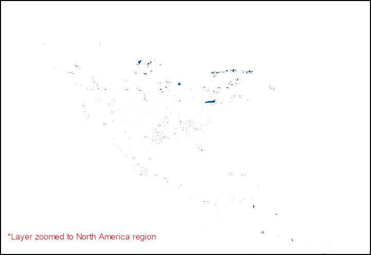

We can also extract a higher resolution extract for a specific region by specifying the extent using the -te option.

gdalwarp -tr 0.005 0.005 -te 68.106 6.762 97.412 37.078 reservoirs.xml reservoirs_india.tif -co COMPRESS=DEFLATE -co TILED=YES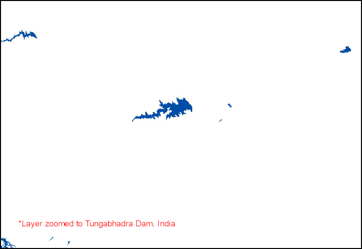

Learn more about offline WMS and comparison between different formats in this article Offline WMS – Benchmarking raster formats for QField by OpenGIS.ch.

Exercise 4

Instead of specifying the resolution in degrees, we want to download the layer at a specific resolution in meters. We can re-project the layer to a projected CRS and specify the output resolution in the units of the target CRS.

Create a command that takes the reservoirs.xml file and creates a GeoTiff file called reservoirs_india_reprojected.tiffor the India region at 500m resolution in the CRS WGS 84 / India NSF LCC (EPSG:7755).

You can use the hints below to construct your command.

• Specify the extent using -te option as 68.106 6.762 97.412 37.078 in the xmin ymin xmax ymax order.
• The extent coordinates are in WGS84 Lat/Lon coordinates. So specify the CRS of the extent coordinates using -te_srs.
• Use the -t_srs option to specify the target CRS as EPSG:7755.
• Use the -tr option to specify the X and Y pixel resolution.

1.6 Georeferencing

GDAL command-line utilities are extremely useful in batch georeferencing tasks. We will learn 2 different techniques for georeferencing/warping images.

1.6.1 Georeferencing Images with Bounding Box Coordinates

Often you get images from web portals that are maps but lack georeferencing information. Data from weather satellites, output from simulations, exports from photo editing software etc. can contain images that reference a fixed frame on the earth but are given in regular image formats such as JPEG or PNG. If the bounding box coordinates and the CRS used in creating these images are known, use gdal_translate command to assign georeference information. The -a_ullr option allows you to specify the bounding box coordinates using the Upper-Left (UL) and Lower-Right (LR) coordinates.

Your data package contains the image file earth_at_night.jpg. This is a beautifully rendered image of the earth captured at night time. You will see that this is a plain JPEG image without any georeference information.

gdalinfo earth_at_night.jpg

Since this is a global image, we know the corner coordinates. We can assign the CRS EPSG:4326 using the -a_srs option and specify the bounding box coordinates in the following order <ulx> <uly> <lrx> <lry>.

Windows

gdal_translate -a_ullr -180 90 180 -90 -a_srs EPSG:4326 ^
  earth_at_night.jpg earth_at_night.tif ^
  -co COMPRESS=JPEG -co TILED=YES -co PHOTOMETRIC=RGB

Mac/Linux

gdal_translate -a_ullr -180 90 180 -90 -a_srs EPSG:4326 \
  earth_at_night.jpg earth_at_night.tif \
  -co COMPRESS=JPEG -co TILED=YES -co PHOTOMETRIC=RGB

The resulting file earth_at_night.tif is a GeoTiff file with the correct georeference information and can now be used in GIS software.

gdalinfo earth_at_night.tif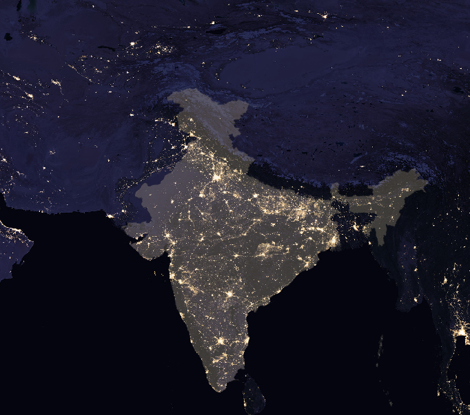

1.6.2 Georeferencing with GCPs

Another option for georeferencing images it by using Ground Control Points (GCPs) or Tie-Points. A GCP specifies the real-world coordinates for a given pixel in the image. The GCPs can be obtained by reading the map markings or locating landmarks from a georeferenced source. Given a set of GCPs, gdalwarp can georeference the image using a variety of transformation types.

Your data package contain an old scanned map called 1870_southern_india.jpg.

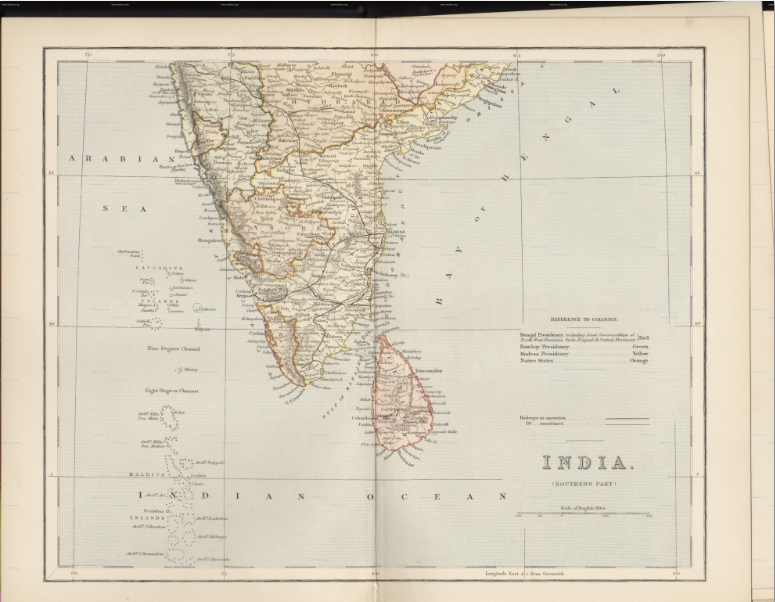
The map has graticule lines with latitude and longitude markings. To obtain the GCPs, we can read the coordinate values at the grid intersections and find the pixel’s image coordinates. You can use an image viewer or the Georeferencer tool in QGIS to obtain GCPs like below.

pixel (column)	line (row)	X (Longitude)	Y (Latitude)
418	893	70	15
380	2432	70	5
3453	2434	90	5
3407	895	90	15
2662	911	85	15

The first step is to store these GCPs in the image metadata using utility gdal_translate.

Windows

gdal_translate -gcp 418 893 70 15 -gcp 380 2432 70 5 -gcp 3453 2434  90 5 ^
  -gcp 3407 895 90 15 -gcp 2662 911 85 15 ^
  1870_southern-india.jpg india-with-gcp.tif

Mac/Linux

gdal_translate -gcp 418 893 70 15 -gcp 380 2432 70 5 -gcp 3453 2434  90 5 \
  -gcp 3407 895 90 15 -gcp 2662 911 85 15 \
  1870_southern-india.jpg india-with-gcp.tif

Now that the GCPs are stored in the image, we are ready to do the georeferencing. Assuming the CRS of the map is a Geographic CRS based on the Everest 1830 datum, we choose EPSG:4042 as the target CRS.

Next, we need to choose the transformation type. gdalwarp supports the following transformation types

• Polynomial 1,2 or 3 using -order option
• Thin Plate Spline using the -tps option

Let’s try Polynomial 1 transformation and check the results.

Windows

gdalwarp -t_srs EPSG:4042 -order 1 -tr 0.005 0.005  ^
  india-with-gcp.tif india-reprojected-polynomial.tif ^
  -co COMPRESS=JPEG -co JPEG_QUALITY=50 -co PHOTOMETRIC=YCBCR

Mac/Linux

gdalwarp -t_srs EPSG:4042 -order 1 -tr 0.005 0.005 \
  india-with-gcp.tif india-reprojected-polynomial.tif \
  -co COMPRESS=JPEG -co JPEG_QUALITY=50 -co PHOTOMETRIC=YCBCR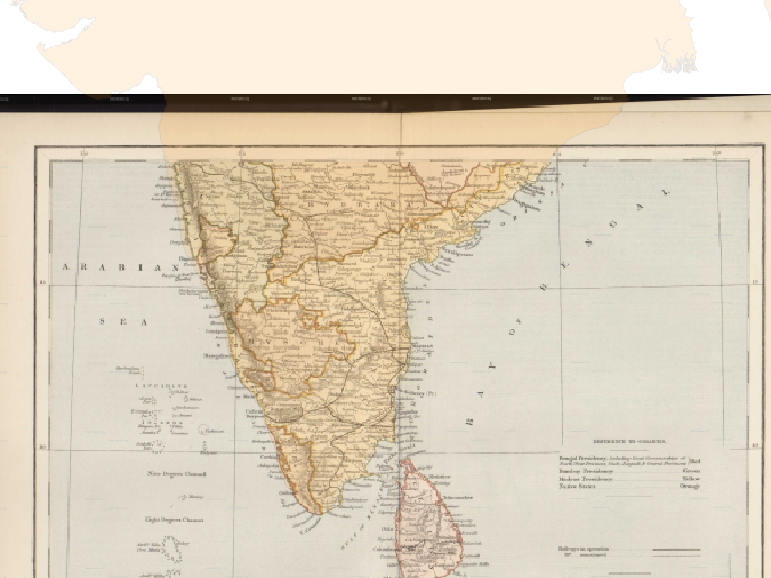

Exercise 5

Try the Thin-plate-spline transformation on the india-with-gcp.tif file and save the results as india-reprojected-tps.tif file. Note the Thin-Place-Splie option is available at -tps with the gdalwarp command.

Assignment

UK’s Department of Environment Food & Rural Affairs (DEFRA) provides country-wide LiDAR data and products via the Defra Data Services Platform under an open license.

Your data package contains a folder london_1m_dsm. This folder contains 1m resolution Digital Surface Model (DSM) tiles for central London generated from a LIDAR survey. The tiles are in the Arc/Info ASCII Grid format with the .asc extension. The tiles do not contain any projection information but the metadata contains the information that the CRS for the dataset is EPSG:27700 British National Grid.

Apply the skills you learnt in this module to create an output product suitable for analysis. The result should be a single georeferenced mosaic in the GeoTIFF format with appropriate compression.

• Hint: Use the gdal_translate program with the -a_srs option to assign a CRS.

2. OGR Tools

We will now learn to process vector data using OGR Tools. These are a suite of tools that are part of the GDAL package and follow the same convention. In addition to format translation, the OGR tools also support running Spatial SQL queries - making them very powerful to build Spatial ETL pipelines.

Start Module Videos ↗

2.1 ETL Basics

In this section, we will see how we can build an Extract-Transform-Load (ETL) process in a step-by-step manner. The example workflow will show you how to

1. Read a CSV data source
2. Convert it to point data layer
3. Assign it a CRS
4. Extract a subset
5. Change the data type of a column
6. Write the results to a GeoPackage.

2.1.1 Read a CSV data source

Your data package has a CSV file called worldcities.csv. This file contains basic information about major cities in the world along with their coordinates.

Let’s use the ogrinfo command to inspect the dataset.

ogrinfo worldcities.csv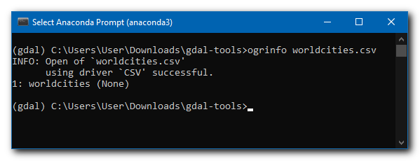

The program can open and read the file successfully, but it doesn’t show any other info. We can use the -al option to actually read all the lines from the file and combine it with the -so option to print a summary.

ogrinfo -so -al worldcities.csv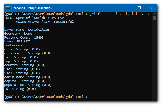

2.1.2 Convert it to point data layer

We now get a summary with the total number of features in the file along with columns and their types. This is a plain CSV file. Let’s turn it into a spatial data layer using the X and Y coordinates supplied in the lng and lat fields. The -oo option allows us to specify format-specific options. The OGR CSV Driver allows specifying a list of column names or a name pattern (such as Lat*) s using the X_POSSIBLE_NAMES and Y_POSSIBLE_NAMES options to specify which columns contain geometry information.

ogrinfo -so -al worldcities.csv -oo X_POSSIBLE_NAMES=lng -oo Y_POSSIBLE_NAMES=lat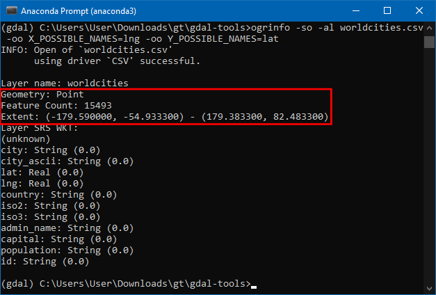

OGR is now able to recognize this layer as Point geometry layer. Let’s write this to a spatial data format. We can use the ogr2ogr utility to translate between different formats. The following command creates a new GeoPackage file called worldcities.gpkg from the CSV file.

Windows

ogr2ogr -f GPKG worldcities.gpkg worldcities.csv ^
  -oo X_POSSIBLE_NAMES=lng -oo Y_POSSIBLE_NAMES=lat 

Mac/Linux

ogr2ogr -f GPKG worldcities.gpkg worldcities.csv \
  -oo X_POSSIBLE_NAMES=lng -oo Y_POSSIBLE_NAMES=lat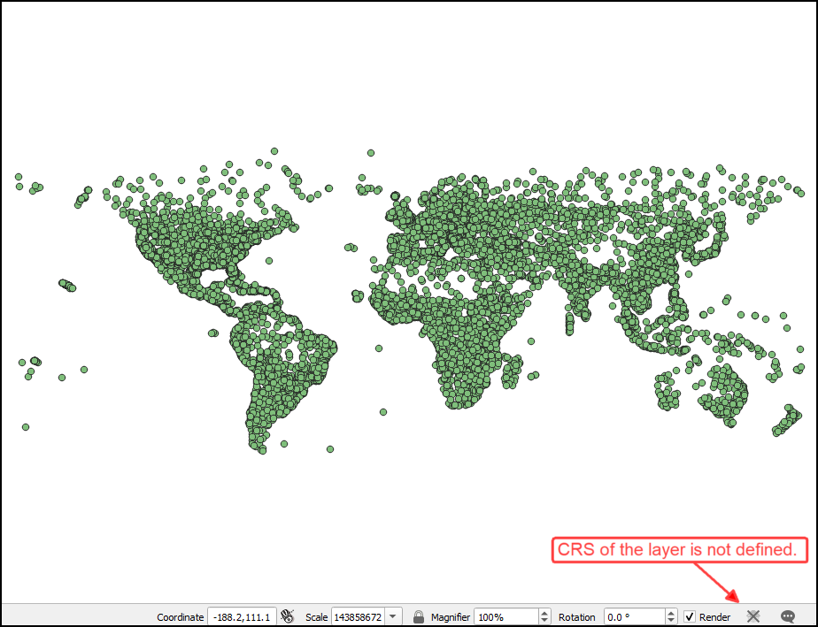 

2.1.3 Assign it a CRS

We can open the result in a GIS software and it shows the cities layer. While the point layer loads fine, it is missing a CRS. We can use the a_srs option to assign a CRS to the resulting layer.

Windows

ogr2ogr -f GPKG worldcities.gpkg worldcities.csv ^
  -oo X_POSSIBLE_NAMES=lng -oo Y_POSSIBLE_NAMES=lat -a_srs EPSG:4326

Mac/Linux

ogr2ogr -f GPKG worldcities.gpkg worldcities.csv \
  -oo X_POSSIBLE_NAMES=lng -oo Y_POSSIBLE_NAMES=lat -a_srs EPSG:4326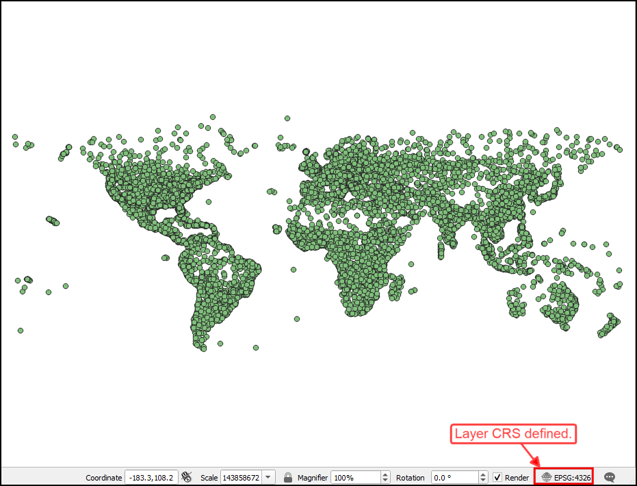

2.1.4 Extract a subset

OGR tools allow executing SQL queries against the data source. It supports a subset of the SQL capability that is described in the OGR SQL Syntax. A simple way to select a subset of features is using the -where option. This allows you to specify an attribute query to filter the results. Here we modify our command to extract only the cities where the country column has the value India.

Windows

ogr2ogr -f GPKG mycities.gpkg worldcities.csv ^
  -oo X_POSSIBLE_NAMES=lng -oo Y_POSSIBLE_NAMES=lat -a_srs EPSG:4326 ^
  -where "country = 'India'"

Mac/Linux

ogr2ogr -f GPKG mycities.gpkg worldcities.csv \
  -oo X_POSSIBLE_NAMES=lng -oo Y_POSSIBLE_NAMES=lat -a_srs EPSG:4326 \
  -where "country = 'India'"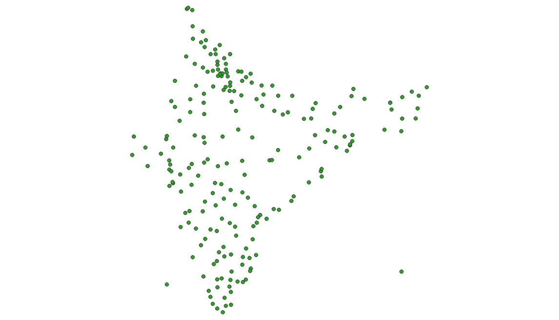

2.1.5 Change the data type of a column

You can also execute any SQL statement on the input data source. This is a very powerful feature that allows you to filter, join, transform, and summarize the input data. We can apply this on our data layer to transform a column type from string to integer. The column population from the input CSV has the type string. Since this field is primarily used to store integer values, we can use the CAST() SQL function to change the type to integer. The SELECT statement also allows us to pick only the relevant fields that will get written to the output.

Windows

ogr2ogr -f GPKG mycities.gpkg worldcities.csv ^
  -oo X_POSSIBLE_NAMES=lng -oo Y_POSSIBLE_NAMES=lat -a_srs EPSG:4326 ^
  -sql "SELECT city, country, CAST(population AS integer) as population ^
    from worldcities where country = 'India'"

Mac/Linux

ogr2ogr -f GPKG mycities.gpkg worldcities.csv \
  -oo X_POSSIBLE_NAMES=lng -oo Y_POSSIBLE_NAMES=lat -a_srs EPSG:4326 \
  -sql "SELECT city, country, CAST(population AS integer) as population \
    from worldcities where country = 'India'"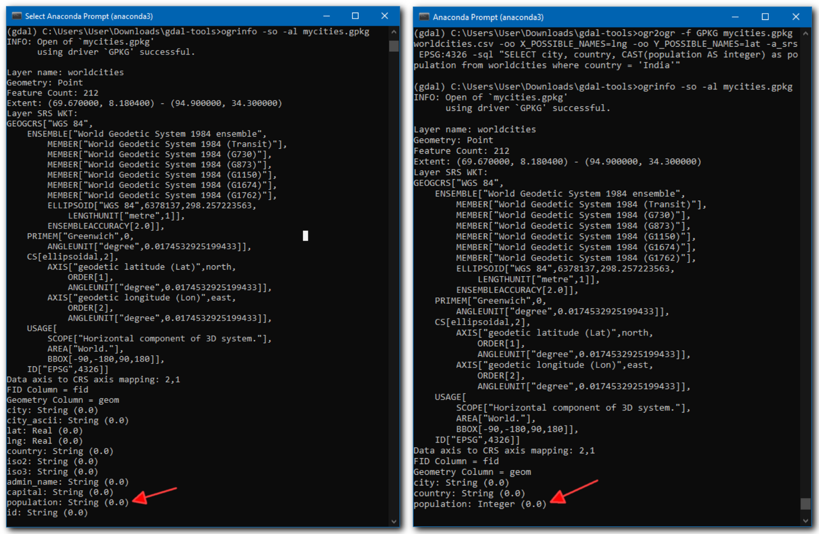

2.1.6 Rename the layer in GeoPackage.

Lastly, we can rename the name of the output layer using the -nln option.

Windows

ogr2ogr -f GPKG mycities.gpkg worldcities.csv ^
  -oo X_POSSIBLE_NAMES=lng -oo Y_POSSIBLE_NAMES=lat -a_srs EPSG:4326 ^
  -sql "SELECT city, country, CAST(population AS integer) as population ^
  from worldcities where country = 'India'" -nln mycities

Mac/Linux

ogr2ogr -f GPKG mycities.gpkg worldcities.csv \
  -oo X_POSSIBLE_NAMES=lng -oo Y_POSSIBLE_NAMES=lat -a_srs EPSG:4326 \
  -sql "SELECT city, country, CAST(population AS integer) as population \
  from worldcities where country = 'India'" -nln mycities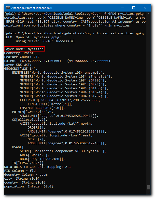

This shows the power of OGR command-line tools. In just a single line, we can read, filter, transform and write the results in any output format supported by OGR.

Exercise 6

Write a command using ogr2ogr that performs the following operations.

• Read the newly created mycities layer from the mycities.gpkg file.
• Reproject the layer to a new CRS EPSG:7755 (WGS84 / India NSF LCC).
• Save the results as a shapefile mycities.shp

All of the above operations should be done in a single-command. Once you arrive at a solution, see if you can improve it by working on the following challenges:

• Challenge 1: You will get a warning that some field values could not be written correctly. This is because the default encoding for the Shapefile format is ISO-8859-1 - which doesn’t support non-latin characters. You can specify the encoding to UTF-8 using the -lco option in ogr2ogr command. Hint: Review the Layer Creation Options for the shapefile driver to see the correct syntax.

• Challenge 2: While you are exploring the Layer Creation Options, add an option to create a spatial index on the output shapefile. Hint: You can specify the -lco option multiple times in the command.

2.2 Merging Vector Files

Another useful utility provided by OGR is ogrmerge.py. This command can merge several vector layers into a single data layer. It also has several options to control how the datasets are merged - making it a very handy tool for data processing tasks.

We will work with several GeoJSON files containing locations of earthquakes. Your data package contains several GEOJSON files in the earthquakes/ directory. We will merge these 12 files into a single file. Switch to the directory

cd earthquakes

We will create a geopackage file by merging all files in the directory. Windows users may need to specify the full path to ogrmerge.py script as follows.

Windows

python %CONDA_PREFIX%\Scripts\ogrmerge.py -o earthquakes.gpkg *.geojson

Mac/Linux

ogrmerge.py -o earthquakes.gpkg *.geojson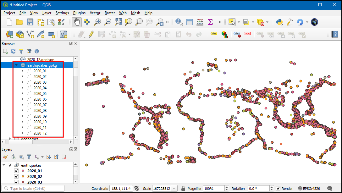

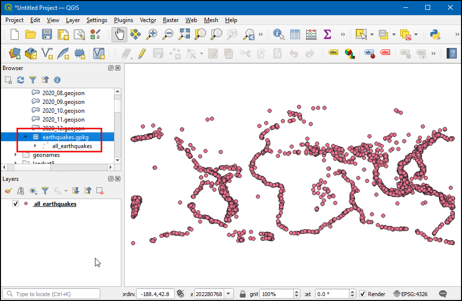
The result will be a single geopackage containing 12 layers - one for each source file. For most applications, it will be preferable to combine source files into a single layer. We can use the -single option to indicate we want a single layer as the output. We also use the -nln option to specify the name of the merged layer. Since the GeoPackage dataset already exists, we need to specify the -overwrite_ds to overwrite the file with the new content.

Windows

python %CONDA_PREFIX%\Scripts\ogrmerge.py -o earthquakes.gpkg *.geojson ^
  -single -nln all_earthquakes -overwrite_ds

Mac/Linux

ogrmerge.py -o earthquakes.gpkg *.geojson \
  -single -nln all_earthquakes -overwrite_ds

Now you will have a single layer named all_earthquakes in the GeoPackage containing all earthquakes recorded during the year.

Tip: There is a very useful option -src_layer_field_name that can add a new field to the output layer containing the name of the input file which contributed that particular record.

Exercise 7

Create a new GeoPackage large_earthquakes.gpkg containing only the earthquakes with magnitude greater than 4.5.

• Use ogr2ogr utility to read the earthquakes.gpkg file created in the previous section.
• Use the -where option to write the query to filter the records where mag field has values greater >4.5.

Challenge: Instead of creating a new geopackage, add a layer named large_earthquakes to the existing earthquakes.gpkg file. Hint: Use the -update option along with -nln to specify the layer name.

2.3 Geoprocessing and Spatial Queries

We have seen examples of using SQL queries in OGR commands. So far we have used the queries that adhere to the OGR SQL Dialect. OGR Tools also have support SQLite dialect. The major advantage of using the SQLite dialect is that you can use Spatial SQL functions provided by Spatialite. This enables a wide range of applications where you can do spatial queries using OGR tools. A major difference when using the SQLite dialect is that you must specify the geometry column explicitly.

Let’s do some geoprocessing and see how we can use spatial queries with OGR Tools. Your data package as a geopackage file spatial_query.gpkg. This geopackage contains 2 layers.

• metro_stations: Point layer with metro rail locations in the city of Melbourne.
• bars_and_pubs: Point layer with locations of bars and pubs in the city of Melbourne.

Let’s see how we can add a new layer to this geopackage with all bars and pubs that are within 500m of a metro station.

2.3.1 Reprojecting Vector Layers

The source data layers are in the CRS EPSG:4326. As we want to run a spatial query with distance in meters, let’s reproject both the layers to a projected CRS. Let’s use the ogr2ogr command to reproject both the input layers and save them into the same geopackage. We can use -t_srs option allows us to specify EPSG:7855 (GDA2020 / MGA Zone 55) as the target projection. the -update option along with -nln tells ogr2ogr to create a new layer and save it in the same geopackage.

Windows

ogr2ogr -t_srs EPSG:7855 spatial_query.gpkg spatial_query.gpkg ^
  bars_and_pubs -update -nln bars_and_pubs_reprojected
ogr2ogr -t_srs EPSG:7855 spatial_query.gpkg spatial_query.gpkg ^
  metro_stations -update -nln metro_stations_reprojected

Mac/Linux

ogr2ogr -t_srs EPSG:7855 spatial_query.gpkg spatial_query.gpkg \
  bars_and_pubs -update -nln bars_and_pubs_reprojected
ogr2ogr -t_srs EPSG:7855 spatial_query.gpkg spatial_query.gpkg \
  metro_stations -update -nln metro_stations_reprojected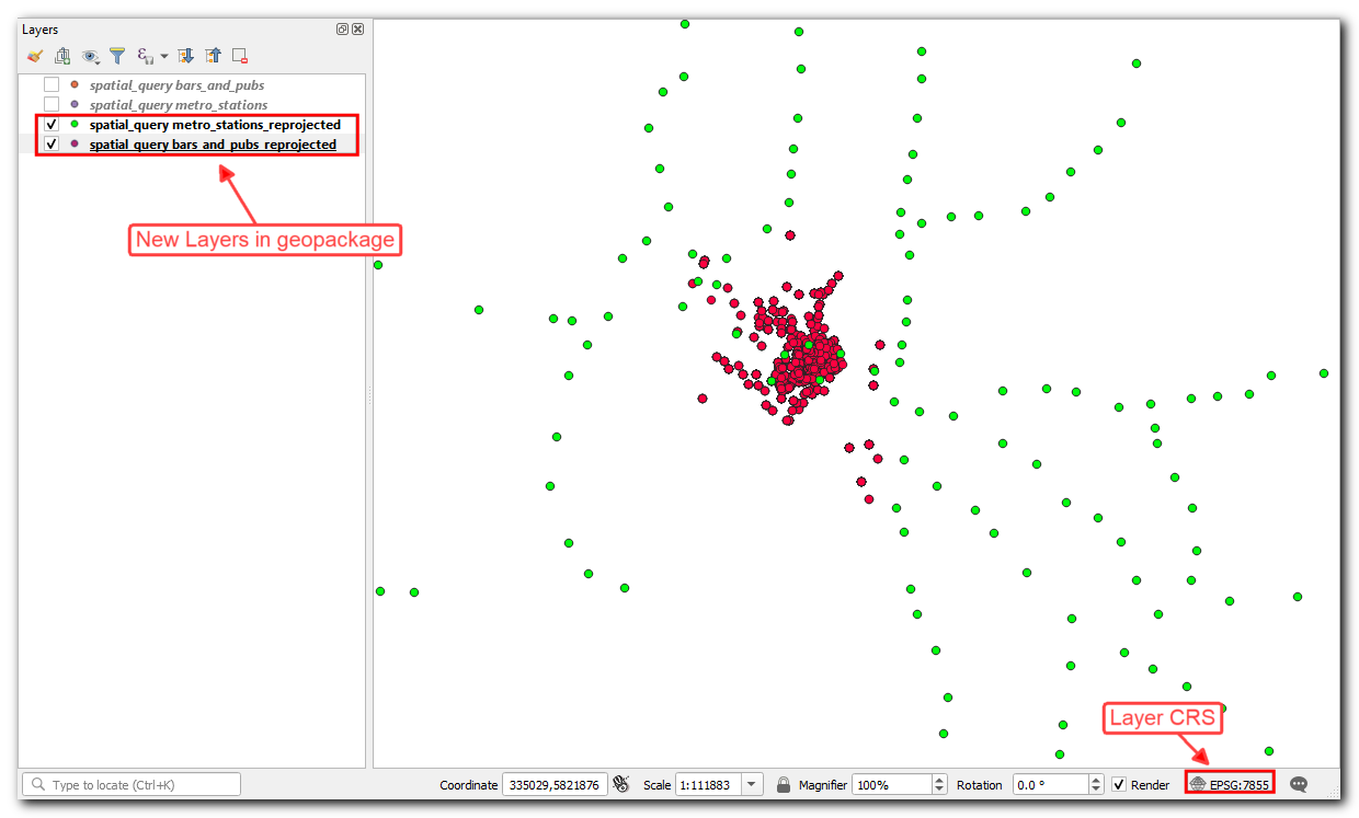

2.3.2 Creating Buffers

Let’s buffer the metro_stations_reprojected layer using a distance of 500 meters. Here we specify the SQL query with the -sql option. Note the use of the ST_Buffer() function which is provided by the Spatialite engine. We need to specify -dialect SQLITE as the query uses spatial functions.

Spatial database functions often have the ST_ prefix. ST stands for Spatial Type.

Windows

ogr2ogr spatial_query.gpkg spatial_query.gpkg -update -nln metro_stations_buffer ^
  -sql "SELECT m.station, ST_Buffer(m.geom, 500) as geom FROM ^
    metro_stations_reprojected m" -dialect SQLITE 

Mac/Linux

ogr2ogr spatial_query.gpkg spatial_query.gpkg -update -nln metro_stations_buffer \
  -sql "SELECT m.station, ST_Buffer(m.geom, 500) as geom FROM \
    metro_stations_reprojected m" -dialect SQLITE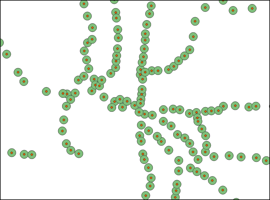 

Metro Station Buffers

This query results in individual overlapping buffers. We can dissolve the buffers using ST_Collect() function.

Windows

ogr2ogr spatial_query.gpkg spatial_query.gpkg -update ^
  -nln metro_stations_buffer_dissolved -sql "SELECT ST_Union(d.geom) as geom ^
    FROM (SELECT ST_Collect(buffer(m.geom, 500)) as geom ^
    FROM metro_stations_reprojected m) as d" -dialect SQLITE

Mac/Linux

ogr2ogr spatial_query.gpkg spatial_query.gpkg -update \
  -nln metro_stations_buffer_dissolved -sql "SELECT ST_Union(d.geom) as geom \
  FROM (SELECT ST_Collect(buffer(m.geom, 500)) as geom \
  FROM metro_stations_reprojected m) as d" -dialect SQLITE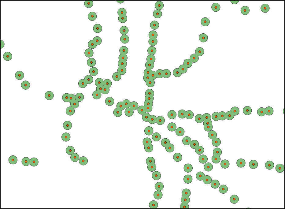

Dissolved Buffers

2.3.3 Performing Spatial Queries

Now that we have a polygon layer with the buffer region around the metro stations, we can use the ogr_layer_algebra.py tool to select the metro stations falling within the buffer region. This tool can perform various types of spatial queries, including Intersection, Difference (Erase), Union etc. We will use the Clip mode to select features from the input layer clipped to the features from the secondary layer.

Windows

python %CONDA_PREFIX%\Scripts\ogr_layer_algebra.py Clip ^
  -input_ds spatial_query.gpkg -input_lyr bars_and_pubs_reprojected ^
  -method_ds spatial_query.gpkg -method_lyr metro_stations_buffer_dissolved ^
  -output_ds output.gpkg -output_lyr selected -nlt POINT

Mac/Linux

ogr_layer_algebra.py Clip \
  -input_ds spatial_query.gpkg -input_lyr bars_and_pubs_reprojected \
  -method_ds spatial_query.gpkg -method_lyr metro_stations_buffer_dissolved \
  -output_ds output.gpkg -output_lyr selected -nlt POINT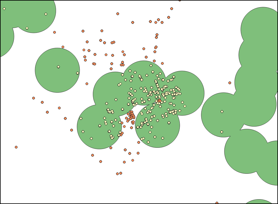

2.3.4 Data Cleaning

The previous query does the job and you find all points that are within the buffer region. But you will notice that there are many duplicate points at the same location. Upon inspecting, you will note that the source data contains multiple features for each establishment from different years. We can run a final SQL query to de-duplicate the data by selecting the feature from the latest year for each establishment. Note that some column names have spaces in the names, so we enclose them in double-quotes.

Windows

ogr2ogr -t_srs EPSG:4326 output.gpkg output.gpkg -update ^
  -nln cleaned -sql "SELECT t1.* FROM selected t1 ^
  JOIN (SELECT \"Property ID\", MAX(\"Census year\") as year FROM selected ^
  GROUP BY \"Property ID\") t2 ON t1.\"Property ID\" = t2.\"Property ID\" ^
  AND t1.\"Census year\" = t2.year"

Mac/Linux

ogr2ogr -t_srs EPSG:4326 output.gpkg output.gpkg -update \
  -nln cleaned -sql "SELECT t1.* FROM selected t1 \
  JOIN (SELECT \"Property ID\", MAX(\"Census year\") as year FROM selected \
  GROUP BY \"Property ID\") t2 ON t1.\"Property ID\" = t2.\"Property ID\" \
  AND t1.\"Census year\" = t2.year"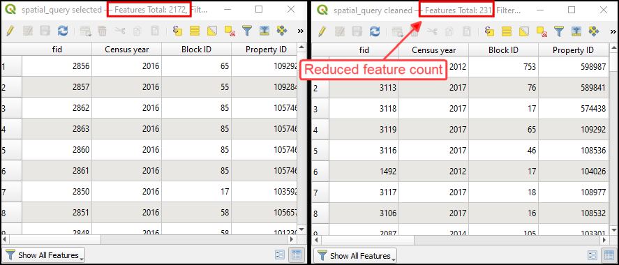

3. Running commands in batch

You can run the GDAL/OGR commands in a loop using Python. For example, if we wanted to convert the format of the images from JPEG200 to GeoTiff for all files in a directory, we would want to run a command like below for every image. Here we want the {input} and {output} values to be determined from the files in a directory.

gdal_translate -of GTiff -co COMPRESS=JPEG {input} {output}

But it would be a lot of manual effort if you want to run the commands on hundreds of input files. Here’s where a simple python script can help you automate running the commands in a batch. The data directory contains a file called batch.py with the following python code.

import os

input_dir = 'naip'

command_string = 'gdal_translate -of GTiff -co COMPRESS=JPEG {input} {output}'
for file in os.listdir(input_dir):
  if file.endswith('.jp2'):
    input = os.path.join(input_dir, file)
    filename = os.path.splitext(os.path.basename(file))[0]
    output =  os.path.join(input_dir, filename + '.tif')
    command = command_string.format(input=input, output=output)
    print('Running ->', command)
    os.system(command)

In Anaconda Prompt, run the following command from gdal-tools directory to start batch processing on all tiles contained in the naip/ directory.

python batch.py

The data directory also contains an example of running the batch commands in parallel using python’s built-in multiprocessing library. If your system has multi-core CPU, running commands in parallel like this on multiple threads can give you performance boost over running them in series.

import os
from multiprocessing import Pool

input_dir = 'naip'
command_string = 'gdal_translate -of GTiff -co COMPRESS=JPEG {input} {output}'

num_cores = 4

def process(file):
    input = os.path.join(input_dir, file)
    filename = os.path.splitext(os.path.basename(file))[0]
    output =  os.path.join(input_dir, filename + '.tif')
    command = command_string.format(input=input, output=output)
    print('Running ->', command)
    os.system(command)
    
files = [file for file in os.listdir(input_dir) if file.endswith('.jp2')]

if __name__ == '__main__':
  p = Pool(num_cores)
  p.map(process, files)

The script runs the commands both in parallel and serial mode and prints the time taken by each of them.

python batch_parallel.py

4. Automating and Scheduling GDAL/OGR Jobs

The easiest way to run commands on a schedule on a Linux-based server is using a Cron Job.

You will have to edit your crontab and schedule the execution of your script (either Shell Script or Python Script). The key is to activate the conda environment before execution of the script.

Assuming you have created a script to execute some GDAL/OGR commands and placed it at /usr/local/bin/batch.py, here’s a sample crontab entry that executes it every morning at 6am.

0 6 * * * conda activate gdal;python /use/local/bin/batch.py; conda deactivate

If you get an error while execution, you may have to include some environment variables in the crontab file so it can find conda correctly. Learn more.

SHELL=/bin/bash
BASH_ENV=~/.bashrc
0 6 * * * conda activate gdal;python batch-parallel.py; conda deactivate

Tips for Improving Performance

Configuration Options

GDAL has several configuration options that can be tweaked to help with faster processing.

• --config GDAL_CACHEMAX 512: This option is the one that helps speed up most GDAL commands by allowing them to use larger amount of RAM (512 MB) reading/writing data.
• --config GDAL_NUM_THREADS ALL_CPUS: This option helps speed up write speed by using multiple threads for compression.
• --debug on: Turn on debugging mode. This prints additional information that may help you find performance bottlenecks.

Multithreading

gdalwarp utility supports multithreaded processing. There are 2 different options for parallel processing.

• -multi: This option parallelizes I/O and CPU operations.
• -wo NUM_THREADS=ALL_CPUS: This option parallelizes CPU operations over several cores.

There is also another option that allows gdalwarp to use more RAM for caching. This option is very helpful to speed up operations on large rasters

• -wm: Set a higher memory for caching

All of these options can be combined that may result in faster processing of the data.

gdalwarp -cutline aoi.shp  -crop_to_cutline naip.vrt aoi.tif -co COMPRESS=DEFLATE -co TILED=YES -multi -wo NUM_THREADS=ALL_CPUS -wm 512 --config GDAL_CACHEMAX 512

Supplement

Check Supported Formats and Capabilities

The GDAL binaries are built to include support for many common data formats. To check what formats are supported in your GDAL distribution, you can run the following command

gdalinfo --formats

Alternatively the --format flag can be used with any other utilities like gdal_translate or ogrinfo to obtain this list.

The output lists the shortnames of all the drivers, whether supports vector or raster data along with abbreviations indicating the capabilities.

Abbreviation	Capabilities
r	read
ro	read only
w	write (create dataset)
w+	write with (support to update)
s	supports subdatasets
v	supports virtual access - eg. /vsimem/

That means an abbreviation of rov indicates that it is a read-only format that supports virtual access.

QGIS distributes versions of GDAL that also has support for non-open formats, such as MrSID. You can use the commands from the included GDAL distribution. The location will depend on the platform and the distribution. Below is an example of how to set the correct path and environment variables for using that.

Open a Command Prompt/Terminal and run the following to set the correct path.

Windows

set OSGEO4W_ROOT=C:\OSGeo4W
call "%OSGEO4W_ROOT%\bin\o4w_env.bat" 
set PATH=%OSGEO4W_ROOT%\bin;%OSGEO4W_ROOT%\apps\qgis-ltr\bin

Mac

export PATH=/Applications/$QGIS_VERSION.app/Contents/MacOS/bin:$PATH

Running gdalinfo --formats will not list MrSID and other proprietary formats.

Extracting Image Metadata and Statistics

You can run gdalinfo command with the -json option which returns the info as a JSON string. This allows you to programatically access the information and parse it.

Let’s say we want to extract the maximum value of the merged.vrt created in the Merging Tiles section. We can get the output of the command as a JSON by supplying the -json option.

gdalinfo -stats -json merged.vrt

Next, we need a way to parse the JSON and extract the fields we are interested in. There are many other command-line utilities designed to do just that. Here we use the popular JSON processing utility jq. You can download and install the jq CLI for your operating system and make sure it is in the system path. Then we can extract the required data using the jq query like below.

gdalinfo -stats -json merged.vrt | jq ".bands[0].maximum"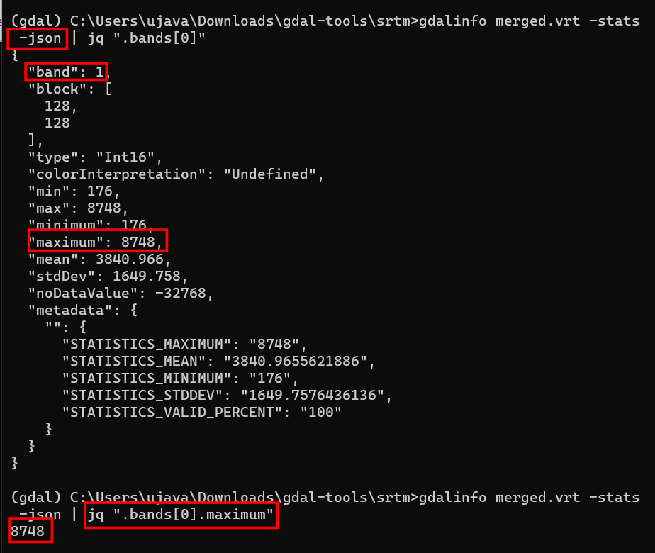

Alternatively, you can also run the command via Python and use the json module to parse and extract the results. The code below shows how to extract the min and max values for each of the SRTM tiles used in the example earlier.

import os
import json
import subprocess

input_dir = 'srtm'

command = 'gdalinfo -stats -json {input}'
for file in os.listdir(input_dir):
  if file.endswith('.hgt'):
    input = os.path.join(input_dir, file)
    filename = os.path.splitext(os.path.basename(file))[0]
    output = subprocess.check_output(command.format(input=input), shell=True)
    info_dict = json.loads(output)
    bands = info_dict['bands']
    for band in bands:
      band_id = band['band']
      min = band['minimum']
      max = band['maximum']
      print('{},{},{},{}'.format(filename, band_id, min, max))

Validating COGs

If you want to check whether a given GeoTIFF file is a valid Cloud-Optimized GeoTIFF (COG) or not, there are several methods.

1. Using the rio command-line utility

Rasterio provides a command-line utility called rio to perform various raster operations on the command-line. The rio-cogeo plugin to Rasterio adds support for creation and validation of COGs.

You can install the required libraries in your conda environment as follows.

conda create --name cogeo
conda activate cogeo
conda install -c conda-forge rasterio rio-cogeo

Once installed, you can validate a COG using the rio cogeo command.

rio cogeo validate merged_cog.tif

This works on cloud-hosted files as well.

rio cogeo validate /vsicurl/https://storage.googleapis.com/spatialthoughts-public-data/ntl/viirs/viirs_ntl_2021_global.tif

2. Using Python

You can use the validate_cloud_optimized_geotiff.py script to check whether a file is a valid COG.

python validate_cloud_optimized_geotiff.py merged_cog.tif

You can also use it in your Python script as follows

import validate_cloud_optimized_geotiff.py
validate_cloud_optimized_geotiff.validate('merged_cog.tif')

Creating Contours

Note : The merged.tif file used below was created in the Merging Tiles section.

The GDAL package comes with the utility gdal_countour that creates contour lines and polygons from DEMs.

You can specify the interval between contour lines using the -i option.

gdal_contour merged.tif contours.gpkg -i 500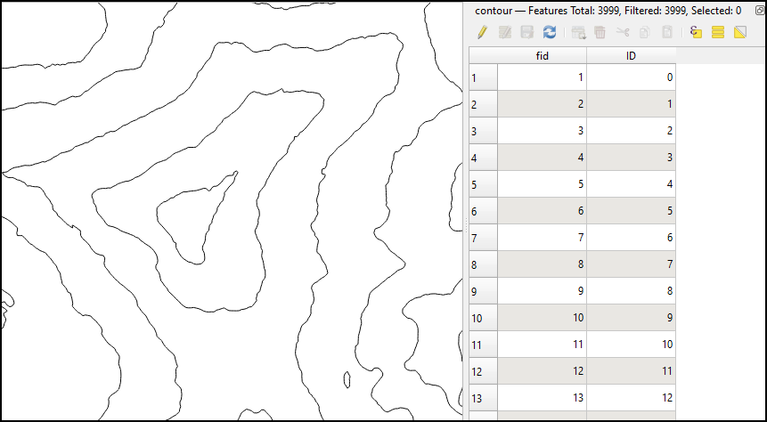

Contour Lines from DEM

Running the command with default options generates a vector layer with contours but they do not have any attributes. If you want to label your contour lines in your map, you may want to create contours with elevation values as an attribute. You can use the -a option and specify the name of the attribute.

gdal_contour merged.tif contours.gpkg -i 500 -a elev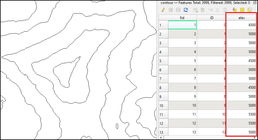

Contour Lines with Elevation Attribute

You can also create polygon contours. Polygon contours are useful in some applications such as hydrology where you want to derive average depth of rainfall in the region between isohyets. You can specify the -p option to create polygon contours. The options -amin and -amax can be provided to specify the attribute names which will store the min and max elevation for each polygon. The command below creates a contour shapefile for the input merged.tif DEM.

gdal_contour merged.tif contour_polygons.shp -i 500 -p -amin MINELEV -amax MAXELEV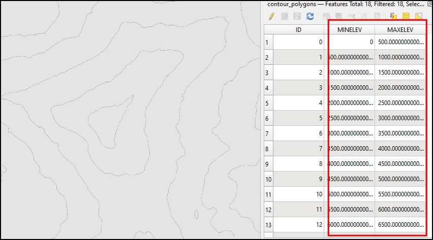

Contour Polygons with Elevation Attributes

Creating Colorized Imagery

We can use gdaldem color-relief command to apply a color palette to any one-band image to create a rendered image.

We create a file ntl_colormap.txt containing the pixel intensity values mapped to RGB colors. The key nv is used to assign a color to NoData values.

0 0 0 4
20 145 43 129
40 251 133 96
50 254 216 154
60 252 253 191
nv 255 255 255

Apply the colormap to the single-band nighttime lights image.

gdaldem color-relief \
  /vsicurl/https://storage.googleapis.com/spatialthoughts-public-data/ntl/viirs/viirs_ntl_2021_india.tif \
  ntl_colormap.txt ntl_colorized.tif

Convert the colorized GeoTIFF to a PNG. Specify the value 255 to set the transparency for the NoData values.

gdal_translate -of PNG -a_nodata 255 ntl_colorized.tif ntl_colorized.png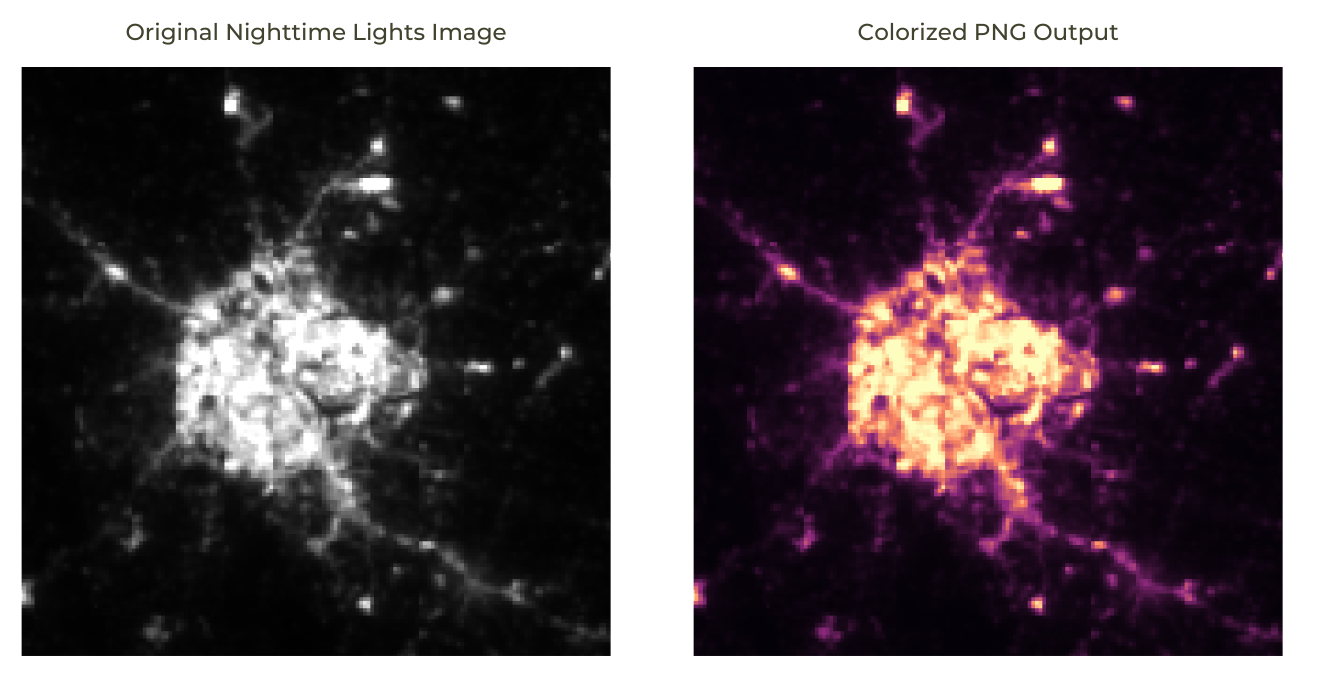

Creating Colorized Hillshade

If you want to merge hillshade and color-relief to create a colored shaded relief map, you can use use gdal_calc.py to create do gamma and overlay calculations to combine the 2 rasters. ¹

gdal_calc.py -A hillshade.tif --outfile=gamma_hillshade.tif \
  --calc="uint8(((A / 255.)**(1/0.5)) * 255)"

gdal_calc.py -A gamma_hillshade.tif -B colorized.tif --allBands=B \
--calc="uint8( ( \
                 2 * (A/255.)*(B/255.)*(A<128) + \
                 ( 1 - 2 * (1-(A/255.))*(1-(B/255.)) ) * (A>=128) \
               ) * 255 )" --outfile=colorized_hillshade.tif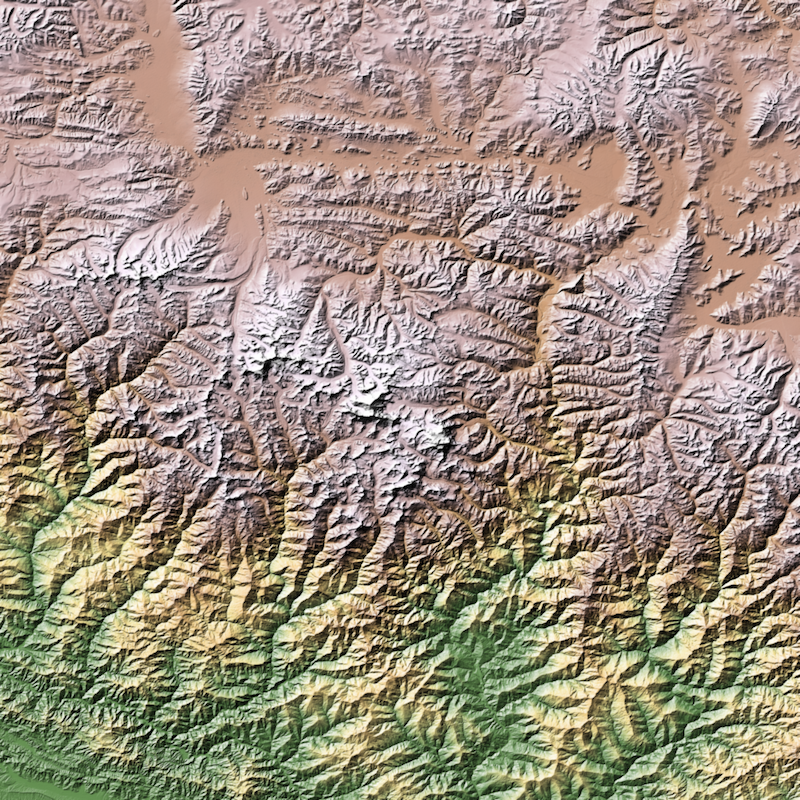

Colorized Shaded Relief

Removing JPEG Compression Artifacts

Applying JPEG compression on aerial or drone imagery can cause the results to have edge artifacts. Since JPEG is a lossy compression algorithm, it causes no-data values (typically 0) being converted to non-zero values. This causes problems when you want to mosaic different tiles, or mask the black pixels. Fortunately, GDAL comes with a handy tool called nearblack that is designed to solve this problem. You can specify a tolerance value to remove edge pixels that may not be exactly 0. It scans the image inwards till it finds these near-black pixel values and masks them. Let’s say we have a mosaic of JPEG compressed imagery without an alpha band and we want to set a mask. If we simply set 0 as nodata value, you will end up with edge artifacts, along with many dark pixels within the mosaic (building shadows/water etc.) being masked. Instead we use the nearblack program to set edge pixels with value 0-5 being considered nodata.

nearblack -near 5 -setmask -o aoi_masked.tif aoi.tif \
  -co COMPRESS=JPEG -co TILED=YES -co PHOTOMETRIC=YCBCR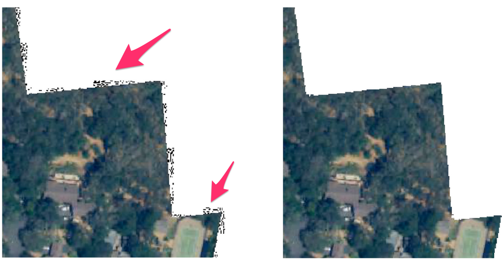

JPEG Artifacts Cleaned by GDAL nearblack

Splitting a Mosaic into Tiles

When delivering large mosaics, it is a good idea to split your large input file into smaller chunks. If you are working with a very large mosaic, splitting it into smaller chunks and processing them independently can help overcome memory issues. This is also helpful to prepare the satellite imagery for Deep Learning. GDAL ships with a handy script called gdal_retile.py that is designed for this task.

Let’s say we have a large GeoTIFF file aoi.tif and want to split it into tiles of 256 x 256 pixels, with an overlap to 10 pixels.

First we create a directory where the output tiles will be written.

mkdir tiles

We can now use the following command to split the file and write the output to the tiles directory.

gdal_retile.py -ps 256 256 -overlap 10 -targetDir tiles/ aoi.tif

This will create smaller GeoTiff files. If you want to train a Deep Learning model, you would typically require JPEG or PNG tiles. You can batch-convert these to JPEG format using the technique shown in the Running Commands in batch section. Since JPEG/PNG cannot hold the georeferencing information, we supply the WORLDFILE=YES creation option.

gdal_translate -of JPEG <input_tile>.tif <input_tile>.jpg -co WORLDFILE=YES

This will create a sidecar file with the .wld extension that will store the georeferencing information for each tile. GDAL will automatically apply the georeferencing information to the JPEG tile as long this file exists in the same directory. This way, you can make inference using the JPG tiles, and use the .wld files with your output to automatically georeference and mosaic the results.

Extracting Projection Information from a Raster

Sometimes you may need to extract and preserve georeferencing information from a raster to be used later or with a different file. A typical use case is Deep Learning - where you need to convert your georeferenced tile (i.e. a GeoTIFF file) into a PNG or JPEG tile. If you used gdal_retile.py as shown in the previous section, you will have a World File accompanying each tile. But many times, you only have the original GeoTIFF file and the resulting PNG tile. To copy the georeferencing information from the GeoTIFF and apply it to the PNG, you can use the following process.

Let’s say we have a georeferenced tile named tile_1_1.tif and a annotated version of this tile from a training dataset as a non-georeferenced tile tile_1_1_annotated.png. We want to georeference this PNG file using the projection and extent of the GeoTIFF file.

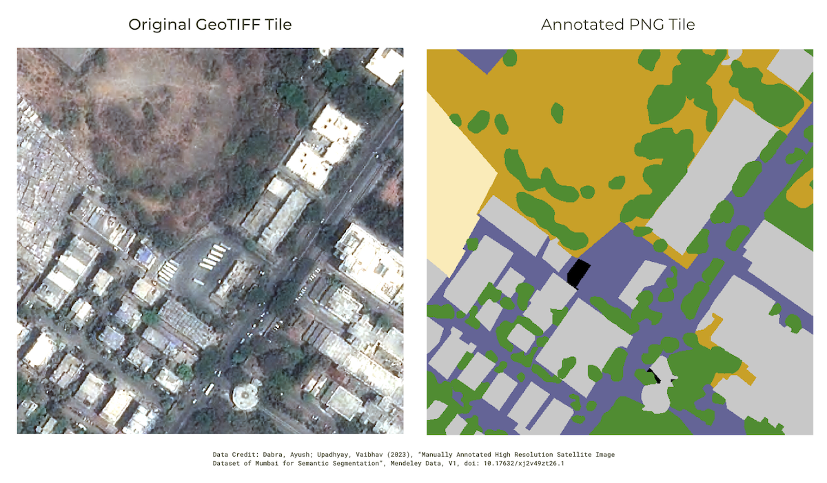
We can extract the extent and resolution of the original GeoTIFF using the listgeo tool. This tool is already part of the standard GDAL conda distribution. We will extract the world file using the -tfw flag that generates an ESRI world file.

listgeo -tfw tile_1_1.tif

You will see that a new file named tile_1_1.tfw is generated alongside the original GeoTIFF. Next we extract the projecton information using gdalsrsinfo command. This command prints the projection information in a variety of supported formats. We save the output to a file with a .prj extension.

gdalsrsinfo tile_1_1.tif > tile_1_1.prj

The tile_1_1.tfw and tile_1_1.prj contain all the information we need to georeference the PNG tile.

Let’s convert the PNG to a GeoTIFF file and assign the projection of the original tile.

gdal_translate -a_srs tile_1_1.prj tile_1_1_annotated.png tile_1_1_annotated.tif

The resulting file contains the projection but the extents are not correct. We can use the geotifcp tool to apply the extents from the world file to the GeoTIFF. This tool is also part of the standard GDAL conda distribution.

geotifcp -e tile_1_1.tfw tile_1_1_annotated.tif tile_1_1_annotated_georeferenced.tif

Merging Files with Different Resolutions

If you had a bunch of tiles that you wanted to merge, but some tiles had a different resolution, you can use specify the -resolution flag with gdalbuildvrt to ensure the output file has the expected resolution.

Continuing the example from the Processing Aerial Imagery section, we can create a virtual raster and specify the resolution flag

gdalbuildvrt -input_file_list filelist.txt naip.vrt -resolution highest -r bilinear

Translating this file using gdal_translate or subsetting it with gdalwarp will result in a mosaic with the highest resolution from the source tiles.

Calculate Pixel-Wise Statistics over Multiple Rasters

gdal_calc.py can compute pixel-wise statistics over many input rasters or multi-band rasters. Starting GDAL v3.3, it supports the full range of numpy functions, such as numpy.average(), numpy.sum() etc.

Here’s an example showing how to compute the per-pixel total from 12 different input rasters. The prism folder in your data package contains 12 rasters of precipitation over the continental US. We will compute pixel-wise total precipitation from these rasters. When you read multiple rasters using the same input flag -A, gdal_calc.py creates a 3D numpy array. It can then be reduced along the axis 0 to produce totals.

cd prism

gdal_calc.py \
    -A PRISM_ppt_stable_4kmM3_201701_bil.bil \
    -A PRISM_ppt_stable_4kmM3_201702_bil.bil \
    -A PRISM_ppt_stable_4kmM3_201703_bil.bil \
    -A PRISM_ppt_stable_4kmM3_201704_bil.bil \
    -A PRISM_ppt_stable_4kmM3_201705_bil.bil \
    -A PRISM_ppt_stable_4kmM3_201706_bil.bil \
    -A PRISM_ppt_stable_4kmM3_201707_bil.bil \
    -A PRISM_ppt_stable_4kmM3_201708_bil.bil \
    -A PRISM_ppt_stable_4kmM3_201709_bil.bil \
    -A PRISM_ppt_stable_4kmM3_201710_bil.bil \
    -A PRISM_ppt_stable_4kmM3_201711_bil.bil \
    -A PRISM_ppt_stable_4kmM3_201712_bil.bil \
    --calc='numpy.sum(A, axis=0)' \
    --outfile total.tif

Currently, gdal_calc.py doesn’t support reading multi-band rasters as a 3D array. So if you want to apply a similar computation on a multi-band raster, you’ll have to specify each band separately. Let’s say, we want to calculate the pixel-wise average value from the RGB composite created in the Merging individual bands into RGB composite section. We can use the command as follows.

gdal_calc.py \
  -A rgb.tif --A_band=1 \
  -B rgb.tif --B_band=2 \
  -C rgb.tif --C_band=3 \
  --calc='(A+B+C)/3' \
  --outfile mean.tif

Extracting Values from a Raster

A useful tool called gdallocationinfo comes with the GDAL suite that can do point lookups from the raster at one or more pairs of coordinates. Combined with GDAL’s capabilities to stream data from cloud datasets with the Virtual File System, you can efficiently lookup pixel values from without having to load the entire raster into memory.

For example, we have a large (8GB) single-band Cloud-Optimized GeoTiff (COG) file on a Google Cloud Storage bucket. This file is a global mosaic of VIIRS Nighttime Lights for the year 2021 and the pixel values are the radiance values.

VIIRS Nighttime Lights 2021

To access this file, we use the /vsigs/ (Google Cloud Storage files) handler and provide the path in form of /vgigs/<bucket_name>/<file_name>. This particular file is public, so we add the config option --config GS_NO_SIGN_REQUEST YES.

gdalinfo /vsigs/spatialthoughts-public-data/ntl/viirs/viirs_ntl_2021_global.tif --config GS_NO_SIGN_REQUEST YES

We are successfully able to open and lookup the metadata of this file. Now let’s query the pixel value at a single coordinate using gdallocationinfo. We specify the location in WGS84 Lon/Lat format, so use the -wgs84 option.

gdallocationinfo -valonly /vsigs/spatialthoughts-public-data/ntl/viirs/viirs_ntl_2021_global.tif -wgs84 77.5946 12.9716 --config GS_NO_SIGN_REQUEST YES

You can also lookup values of multiple points from a file. Let’s say we have a text file called coordinates.txt with the following 2 coordinates.

77.5946 12.9716
77.1025 28.7041

We can lookup the pixel values at these coordinates by supplying this to the gdallocationinfo command. We also supply the -xml option so the output is structured and can be used for post processing.

cat coordinates.txt | gdallocationinfo /vsigs/spatialthoughts-public-data/ntl/viirs/viirs_ntl_2021_global.tif \
  -wgs84 --config GS_NO_SIGN_REQUEST YES -xml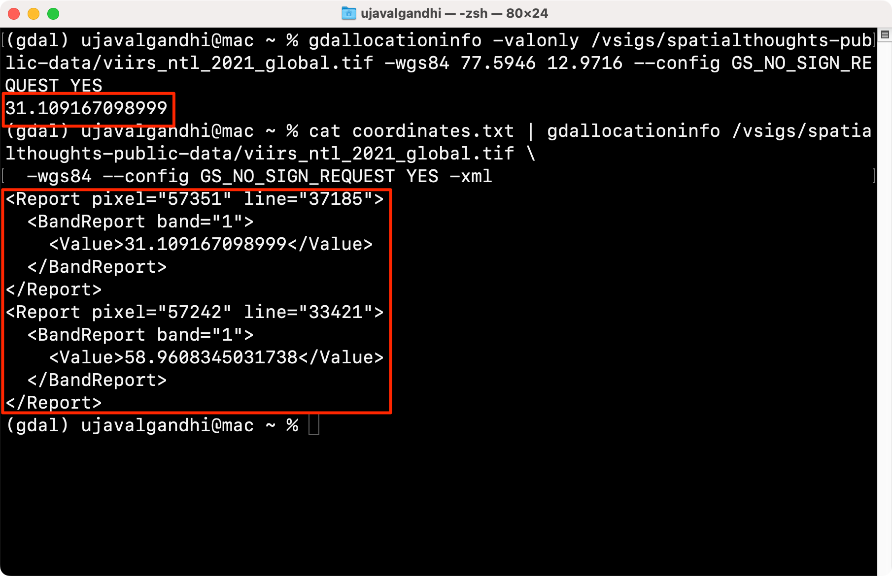

Querying single or multiple values

Masking Values using a Binary Raster

Often we have binary images representing a data mask. We can use numpy.where() function with gdal_calc.py to mask pixels from any raster with a mask image.

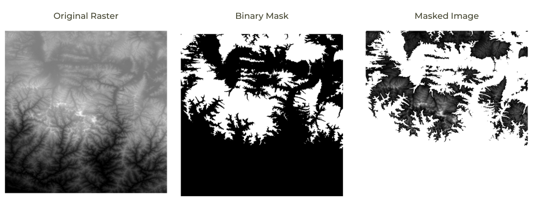
Let’s say we have a binary.tif containing pixel values 0 and 1. We now want to set all pixels from merged.tif to No Data where the binary.tif is 0. Assuming, we want to use -32768 as the No Data value, we can use a command like below.

gdal_calc.py -A merged.tif -B binary.tif \
  --calc="numpy.where(B==1, A, -32768)" \
  --NoDataValue -32768 --outfile masked.tif

This command says Wherever the value of B raster is 1, the output should be the pixel values from A else it should be -32768. Since we are also setting the -NoDataValue to -32768, the command effectively sets all pixels where the condition doesn’t match (B != 1) to NoData.

Raster to Vector Conversion

GDAL comes with the gdal_polygonize.py allowing us to convert rasters to vector layers. Let’s say we want to extract the coordinates of the highest elevation from the merged raster in the Merging Tiles section. Querying the raster with gdalinfo -stats shows us that the highest pixel value is 8748.

We can use gdal_calc.py to create a raster using the condition to match only the pixels with that value.

gdal_calc.py --calc 'A==8748' -A merged.vrt --outfile everest.tif --NoDataValue=0

The result of a boolean expression like above will be a raster with 1 and 0 pixel values. As we set the NoData to 0, we only have 1 pixel with value 1 where the condition matched. We can convert it to a vector using gdal_polygonize.py.

gdal_polygonize.py everest.tif everest.shp

If we want to extract the centroid of the polygon and print the coordinates, we can use ogrinfo command.

ogrinfo everest.shp -sql 'SELECT AsText(ST_Centroid(geometry)) from everest' -dialect SQLite

Viewshed Analysis

The gdal_viewshed command can do visibility analysis using elevation rasters. This is a very useful analysis for many applications including urban planning and telecommunications. We can take the London 1m DSM dataset and carry out the visibility analysis from a location.

We will determine all the areas of London that are visible from the top of the Tower 42 building. This is a skyscraper located in the city of London.

We take the merged DSM created for Assignment 1 and generate a viewshed.

The CRS of the dataset is EPSG:27700 so we need to get the observer location coordinates in this CRS. We can use the gdaltransform command to convert the Lat/Lon coordinates to the coordinates in the target CRS. Run the command below and press enter.

gdaltransform -s_srs EPSG:4326 -t_srs EPSG:27700

The command takes input from the terminal. Enter the X and Y coordinate as follows

-0.083738 51.515178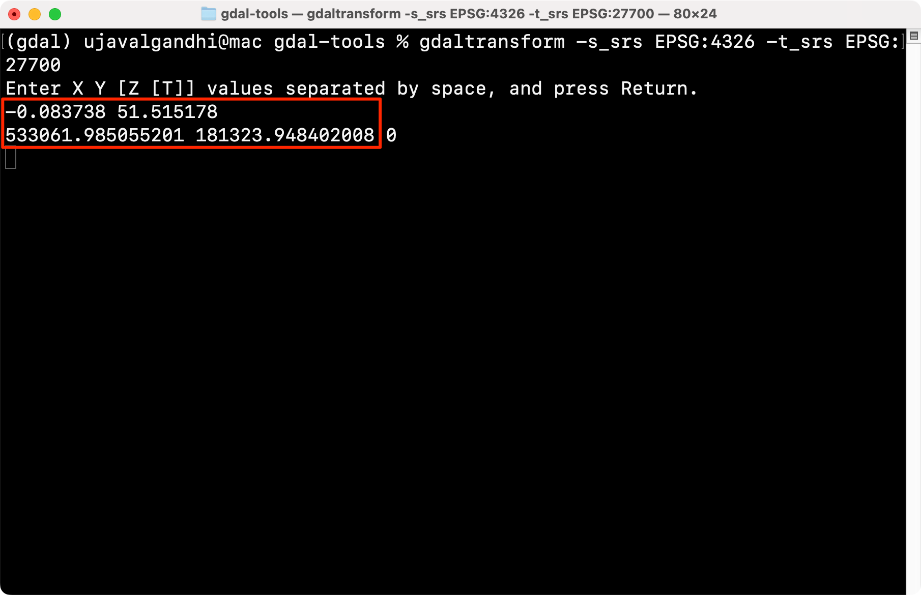

Results of Viewshed Analysis

The output of the command are the X and Y coordinates 533061.985055201 181323.948402008. We round them off and use it in the gdal_viewshed command.

gdal_viewshed -b 1 -ox 533062 -oy 181324 -oz 10 -md 100000.0 -f GTiff -co COMPRESS=DEFLATE -co PREDICTOR=2 merged.tif viewshed_tower42.tif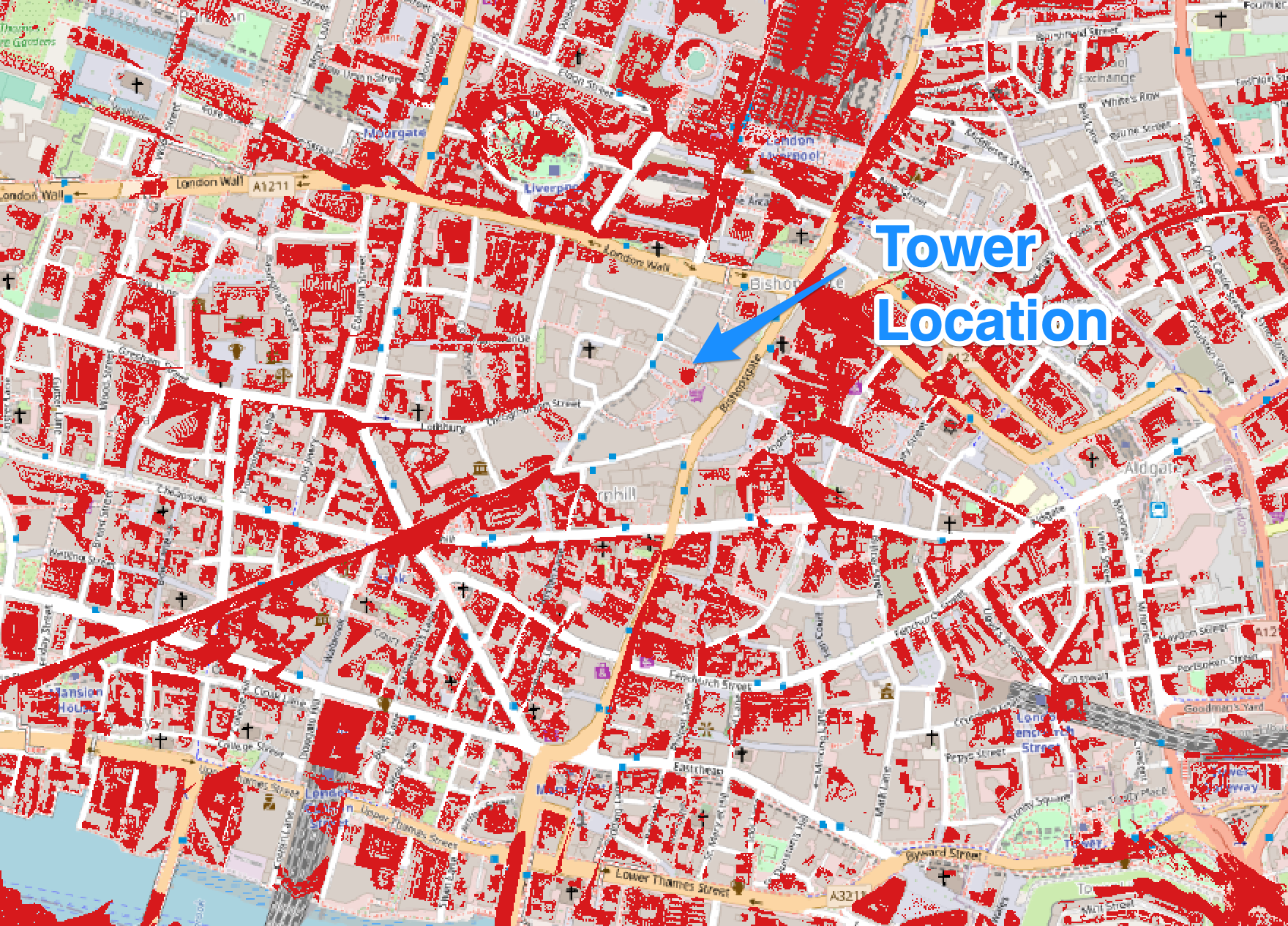

Results of Viewshed Analysis

Working with KML Files

Keyhole Markup Language (KML) is a XML-based file format primarily used by Google Earth. Often time, GIS users want to export their data to KML for visualizing it in Google Earth. You may also want to extract data from KML files or convert them into other spatial formats used in GIS. The GDAL KML Driver can both read and write KML files and provides many options to make the conversion compatible.

Exporting Data to KML files

Let’s take the metro_stations layer from the spatial_query.gpkg file in your data package and export it to a KML file metro_stations.kml.

ogr2ogr -f KML metro_stations.kml spatial_query.gpkg metro_stations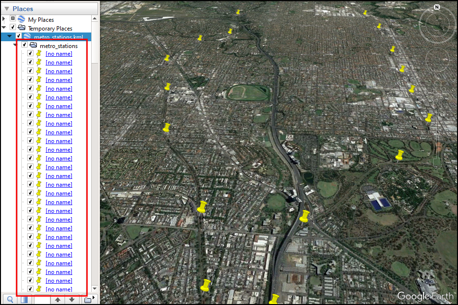 

KML Export without NameField

While the above command works, you will notice that when you open the resulting file in Google Earth, the placemarks for each feature doesn’t have any labels. This is because the KML format expects a field called Name in the layer which is used as the label for each placemark. If your data layer does not have such a field, you can supply an alternate field name that will be used as labels using the -dsco option. The metro_stations layer has a field named station which we can use as the name field.

ogr2ogr -f KML metro_stations.kml spatial_query.gpkg metro_stations -dsco NameField=station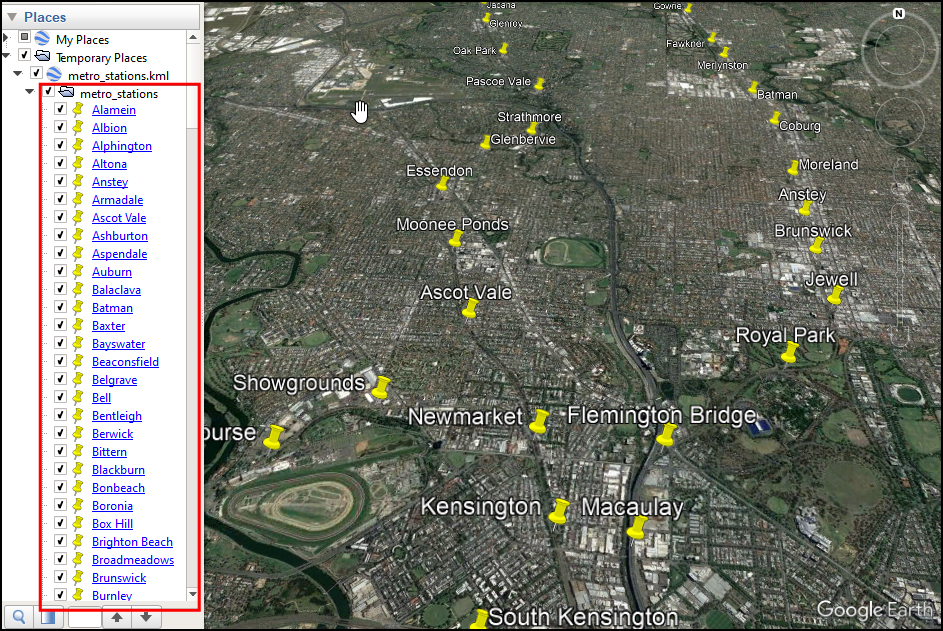

KML Export with NameField

Converting KML Files to Other Formats

The KML file format supports having multiple data layers within the same KML file. We will now learn how to extract a specific data layer and convert it to a shapefile. GDAL supports reading data from a URL using the Virtual File System. We can read a KML file from the internet using the vsicurl/ prefix.

ogrinfo /vsicurl/https://developers.google.com/kml/documentation/KML_Samples.kml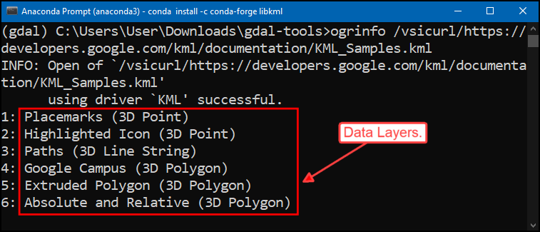

Let’s read the Paths layer

ogrinfo /vsicurl/https://developers.google.com/kml/documentation/KML_Samples.kml Paths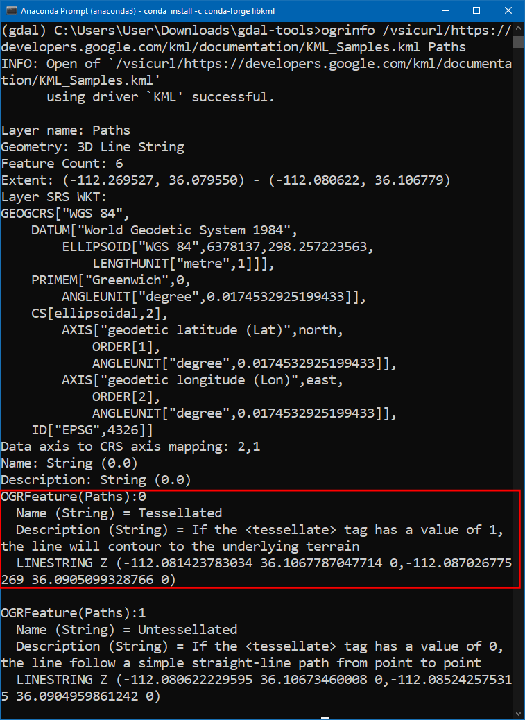

To extract the Paths layer from this KML file, we can use ogr2ogr command. The default options create many unwanted fields in the output. We can select a subset of the input fields using the -select option.

ogr2ogr -f "ESRI Shapefile" paths.shp /vsicurl/https://developers.google.com/kml/documentation/KML_Samples.kml Paths -select "NAME,Description"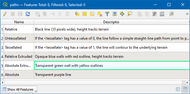

You can also convert a KML layer to a CSV file. The GDAL CSV Driver is able to extract the geometry of features using the GEOMETRY layer creation option. Let’s convert the Placemark layer from the KML_Samples.kml to a CSV file with X, Y and Z columns extracted from the geometry.

ogr2ogr -f CSV points.csv /vsicurl/https://developers.google.com/kml/documentation/KML_Samples.kml Placemarks -lco GEOMETRY=AS_XYZ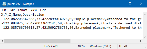

KML vs. LIBKML Drivers

If your GDAL binaries are compiled with support for the LIBKML Driver, it is preferable to use it over the KML driver. The LIBKML driver supports many more options and allows you to create fully featured KMLs.

Below is an example of data conversion using the LIBKML driver. To specify the name field, the LIBKML driver uses an environment variable called LIBKML_NAME_FIELD that can be specified with the --config option

ogr2ogr -f LIBKML metro_stations.kml spatial_query.gpkg metro_stations --config LIBKML_NAME_FIELD station

If your GDAL version has both KML and LIBKML drivers, OGR will prefer the LIBKML driver. To force OGR to use the KML driver for reading files, you can add --config OGR_SKIP LIBKML to your command.

Group Statistics

We can use SQL GROUP BY clause in ogr2ogr to generate summary statistics from a layer. Let’s first create a geopackage from the worldcities.csv layer.

ogr2ogr -oo X_POSSIBLE_NAMES=lng -oo Y_POSSIBLE_NAMES=lat -a_srs EPSG:4326 \
  -sql "SELECT city, country, CAST(population as integer) as population from worldcities" \
  worldcities.gpkg worldcities.csv -nln worldcities

We have a layer worldcities.gpkg that has population and country columns. Let’s calculate the total population per country. We can save the resulting statistics as an Excel sheet.

ogr2ogr stats.xlsx worldcities.gpkg \
  -sql "SELECT country, sum(population) as total_population from worldcities GROUP BY country"

Using Virtual Layers

Similar to GDAL, OGR also supports Virtual File Format (VRT). Compared to the raster version, the OGR Virtual Driver is much more capable and can be used for on-the-fly data transformations. Multiple data layers can be combined into a single virtual layer using the XML-based .vrt format files. VRT files are also used to configure reading tabular data into spatial data formats.

Read Geonames Files

Your data package contains 3 large text files from Geonames in the geonames folder. These are plain-text files in a Tab-Separated Values (TSV) format. Change to the geonames directory.

cd geonames

Let’s try reading one of the files CA.txt - which has over 300K records of all placenames in Canada. To read this file, we need to create a new file called CA.vrt with the following content. Save the file in the same geonames directory.

<OGRVRTDataSource>
        <OGRVRTLayer name="CA">
            <SrcDataSource>CSV:CA.txt</SrcDataSource>
            <SrcLayer>CA</SrcLayer>
        </OGRVRTLayer>
</OGRVRTDataSource>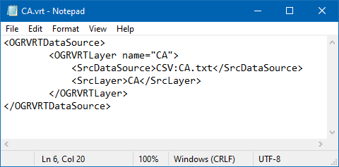

Let’s check if OGR can read the source text file via the newly created CA.vrt file.

ogrinfo -al -so CA.vrt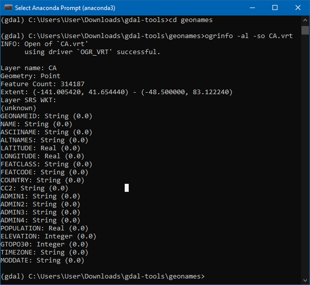

The ogrinfo command was able to successfully read the data and show us the summary of the attributes as well as the total feature count. Note that OGR has built-in support for the geonames file format. So it was able to correctly detect the geometry columns without us specifying it. For other datasets, you will have to specify the geometry columns explicitly via the <GeometryField> attribute in the VRT file.

Applying Filters

VRT format supports applying SQL queries on the source layer using the <SrcSQL> field. This allows us to create an on-the-fly filter that reads only a subset of the data. Update the CA.vrt with the following content.

<OGRVRTDataSource>
        <OGRVRTLayer name="CA">
            <SrcDataSource>CSV:CA.txt</SrcDataSource>
            <SrcLayer>CA</SrcLayer>
            <SrcSQL>select * from CA where "FEATCLASS" = 'T'</SrcSQL>
        </OGRVRTLayer>
</OGRVRTDataSource>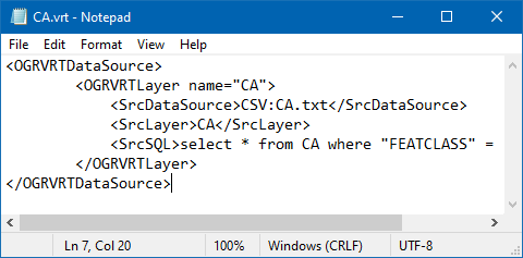

The VRT file now contains a SQL query to select only the mountain features from the source file. Let’s run ogrinfo again and check the output.

ogrinfo -al -so CA.vrt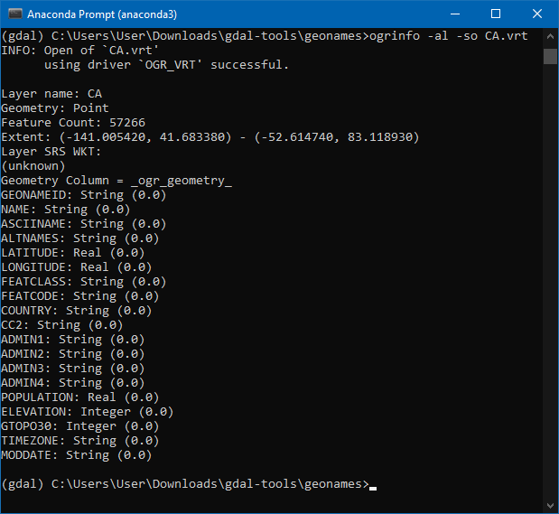

You will see that the output contains a subset of features, even though we never changed the source data.

Merging Files

The real power of the VRT file format lies in its ability to dynamically combine multiple data sources into a single data layer. We can adapt the previously created file and use <OGRVRTUnionLayer> to create a single layer from the 3 separate text files. Save the following content into a new file named NA.vrt.

<OGRVRTDataSource>
    <OGRVRTUnionLayer name="NA">
    
        <OGRVRTLayer name="CA">
            <SrcDataSource>CSV:CA.txt</SrcDataSource>
            <SrcLayer>CA</SrcLayer>
            <SrcSQL>select * from CA where "FEATCLASS" = 'T'</SrcSQL>
        </OGRVRTLayer>
    
        <OGRVRTLayer name="MX">
            <SrcDataSource>CSV:MX.txt</SrcDataSource>
            <SrcLayer>MX</SrcLayer>
            <SrcSQL>select * from MX where "FEATCLASS" = 'T'</SrcSQL>
        </OGRVRTLayer>
    
        <OGRVRTLayer name="US">
            <SrcDataSource>CSV:US.txt</SrcDataSource>
            <SrcLayer>US</SrcLayer>
            <SrcSQL>select * from US where "FEATCLASS" = 'T'</SrcSQL>
        </OGRVRTLayer>
    
    </OGRVRTUnionLayer> 
</OGRVRTDataSource>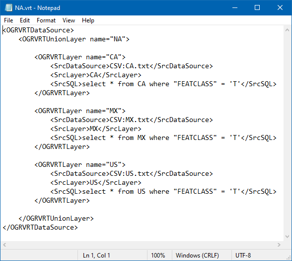

Let’s now translate the NA.vrt to a GeoPackage using the ogr2ogr command.

ogr2ogr -f GPKG NA.gpkg NA.vrt -a_srs EPSG:4326

This operation requires a lot of processing and may take a few minutes. You can add the --config GDAL_CACHEMAX 512 option to speed up the process. See Tips for Improving Performance section for more details.

This command reads all 3 text files, filters them for matching features, combines them and writes out a spatial layer containing all mountains in North America.

Resources

• GDAL Tips @gdaltips on Twitter
• A Gentle Introduction to GDAL by Robert Simmon Part-1, Part-2, Part-3, Part-4, Part-5, Part-6, Part-7
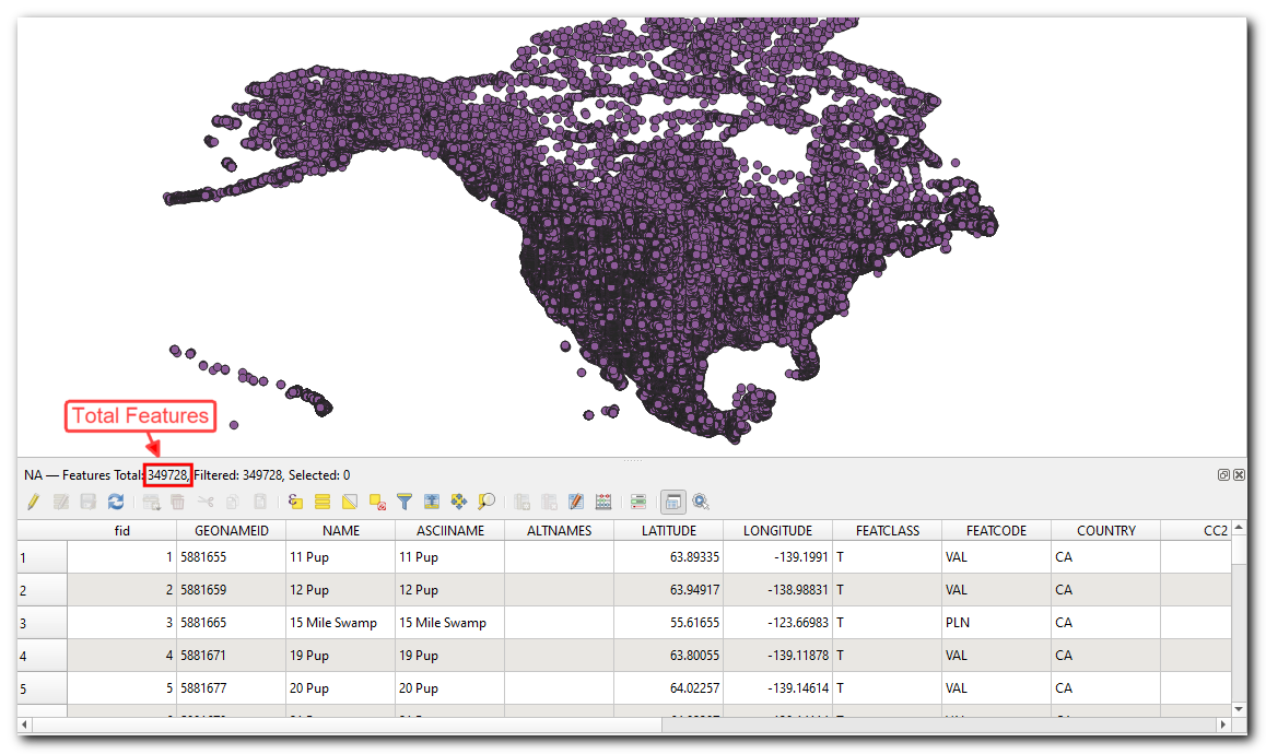
• Data Science at the Command Line by Jeroen Janssens

Data Credits

• Landsat: Landsat-8 image courtesy of the U.S. Geological Survey. Image downloaded from Google Cloud Platform and pre-processed using Semi Automatic Classification Plugin from QGIS
• Earth at Night image: Credit: NASA Earth Observatory/NOAA NGDC. Earth at Night flat hi-resolution map downloaded from NASA earth observatory
• William Mackenzie 1870 map of Southern India: out-of-copyright scanned map downloaded from Hipkiss’s Scanned Old Maps
• NAIP 2016 Aerial Imagery for California: The National Agriculture Imagery Program (NAIP). USDA-FSA-APFO Aerial Photography Field Office. Downloaded from NRCS
• London 1m DSM. Downloaded from Defra Data Services Platform. © Environment Agency copyright and/or database right 2019. All rights reserved.
• Melbourne Metro Stations: © 2019 The City of Melbourne Open Data Portal. Data provided by Metro Trains Melbourne
• Melbourne Bars and Pubs: © 2019 The City of Melbourne Open Data Portal. Data provided by Census of Land Use and Employment (CLUE)
• VIIRS Annual VNL V2 for 2021. C. D. Elvidge, M. Zhizhin, T. Ghosh, F-C. Hsu, “Annual time series of global VIIRS nighttime lights derived from monthly averages: 2012 to 2019”, Remote Sensing (In press)

License

This course material is licensed under a Creative Commons Attribution-NonCommercial 4.0 International License. You are free to use the material for any non-commercial purpose. Kindly give appropriate credit to the original author.

If you would like to utilize these materials as part of a commercial offering, you can purchase a Trainer License for a small fee.

Please contact us for pricing and terms.

© 2020 Ujaval Gandhi www.spatialthoughts.com

---

This course is offered as an instructor-led online class. Visit Spatial Thoughts to know details of upcoming sessions.

---

1. Code reference https://gis.stackexchange.com/questions/255537/merging-hillshade-dem-data-into-color-relief-single-geotiff-with-qgis-and-gdal↩︎

---

If you want to report any issues with this page, please comment below.