Introduction
Sign-up for Google Earth Engine
Get the Course Materials
1. Reducers
Joins
Regressions
Vector Data Processing and Visualization
License
Citing and Referencing

Introduction

This is an advanced-level course that is suited for participants who are familiar with the Google Earth Engine API and want to learn advanced data processing techniques and understand the inner-workings in Earth Engine. This class covers the following topics:

Reducers
Joins (coming soon)
Regressions (coming soon)
Vector Data Processing and Visualization (coming soon)

Get the Course Materials

The course material and exercises are in the form of Earth Engine scripts shared via a code repository.

Click this link to open Google Earth Engine code editor and add the repository to your account.
If successful, you will have a new repository named users/ujavalgandhi/GEE-Advanced in the Scripts tab in the Reader section.
Verify that your code editor looks like below

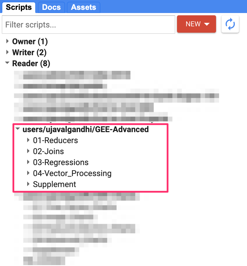
Code Editor with Workshop Repository

If you do not see the repository in the Reader section, click Refresh repository cache button in your Scripts tab and it will show up.

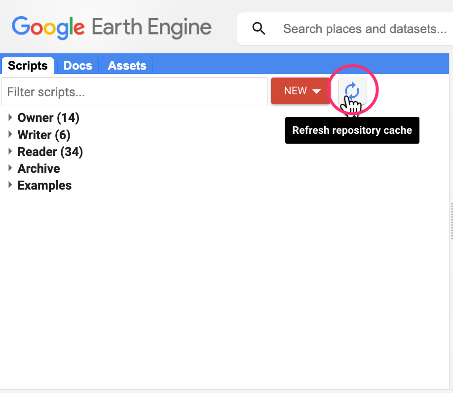
Refresh repository cache

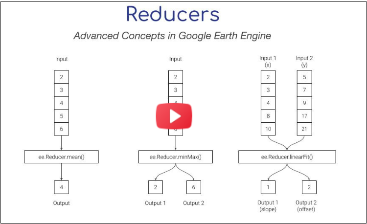
1. Reducers

Reducer is an object used to compute statistics or perform aggregations. Reducers can aggregate data over time, space, bands, lists and other data structures in Earth Engine. Each reducer can take one or more input and generate one of more outputs.

View the Presentation ↗

This module is also available as video.

Watch Video

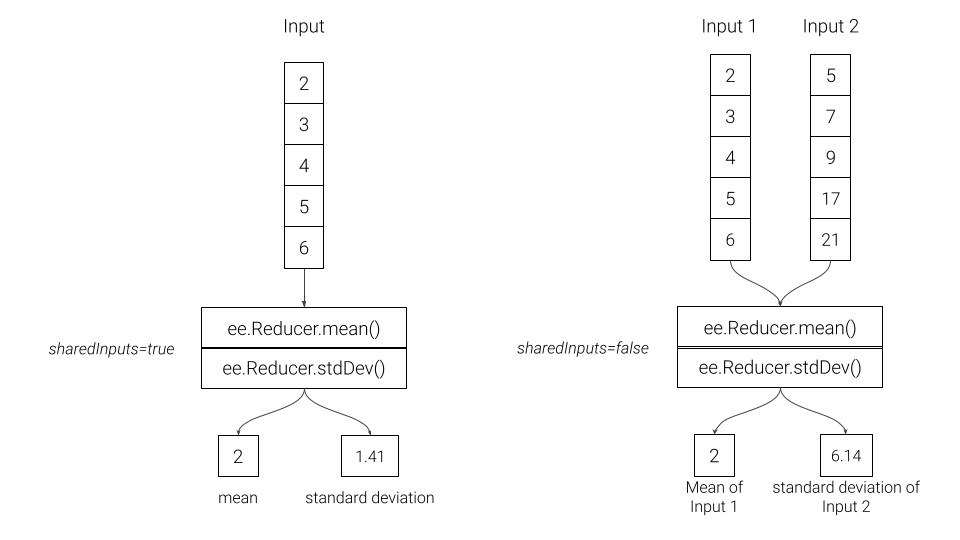
01. Combined Reducers

You can create a new reducer by combining multiple reducers. Combined reducers are useful to compute multiple statistics together. The resulting reducer is run in parallel and is highly efficient than running each reducer independently.

Combined Reducers

Open in Code Editor ↗

// Example script showing how to extract data
// from images and imagecollections
var admin2 = ee.FeatureCollection('FAO/GAUL_SIMPLIFIED_500m/2015/level2');
var admin2Filtered = admin2.filter(ee.Filter.eq('ADM2_NAME', 'Bangalore Urban'));
var geometry = admin2Filtered.geometry();

// We use the MODIS 16-day Vegetation Indicies dataset
var modis = ee.ImageCollection('MODIS/061/MOD13Q1');

// Pre-Processing: Cloud Masking and Scaling

// Function for Cloud Masking
var bitwiseExtract = function(input, fromBit, toBit) {
  var maskSize = ee.Number(1).add(toBit).subtract(fromBit)
  var mask = ee.Number(1).leftShift(maskSize).subtract(1)
  return input.rightShift(fromBit).bitwiseAnd(mask)
}

var maskSnowAndClouds = function(image) {
  var summaryQa = image.select('SummaryQA')
  // Select pixels which are less than or equals to 1 (0 or 1)
  var qaMask = bitwiseExtract(summaryQa, 0, 1).lte(1)
  var maskedImage = image.updateMask(qaMask)
  return maskedImage.copyProperties(
    image, ['system:index', 'system:time_start'])
}

// Function for Scaling Pixel Values
// MODIS NDVI values come as NDVI x 10000
// that need to be scaled by 0.0001
var ndviScaled = function(image) {
  var scaled = image.divide(10000)
  return scaled.copyProperties(
    image, ['system:index', 'system:time_start'])
};

// Apply the functions and select the 'NDVI' band
var processedCol = modis
  .map(maskSnowAndClouds)
  .map(ndviScaled)
  .select('NDVI');

// Extracting Image Statistics

var startDate = ee.Date.fromYMD(2019, 1, 1);
var endDate = startDate.advance(1, 'year')

var filtered = processedCol
  .filter(ee.Filter.date(startDate, endDate))

var image = filtered.mean();

Map.addLayer(geometry, {}, 'Region');
Map.addLayer(image.clip(geometry), {min:0, max:1, palette:['#FFFFFF', '#006400']}, 'MODIS NDVI')
Map.centerObject(geometry);

// Compute Mean NDVI
var stats = image.reduceRegion({
    reducer: ee.Reducer.mean(),
    geometry: geometry,
    scale: 250
});
print('Mean NDVI', stats.getNumber('NDVI'));

// Use a Combined Reducer
var stats = image.reduceRegion({
    reducer: ee.Reducer.mean().combine({
      reducer2: ee.Reducer.minMax(),
      sharedInputs: true}),
    geometry: geometry,
    scale: 250
});
print('NDVI Statistics', stats);

// You can combine as many reducers as you want
var allReducers = ee.Reducer.mean()
  .combine({reducer2: ee.Reducer.min(), sharedInputs: true} )
  .combine({reducer2: ee.Reducer.max(), sharedInputs: true} )
  .combine({reducer2: ee.Reducer.percentile([25]), sharedInputs: true} )
  .combine({reducer2: ee.Reducer.percentile([50]), sharedInputs: true} )
  .combine({reducer2: ee.Reducer.percentile([75]), sharedInputs: true} )

var stats = image.reduceRegion({
    reducer: allReducers,
    geometry: geometry,
    scale: 250
});
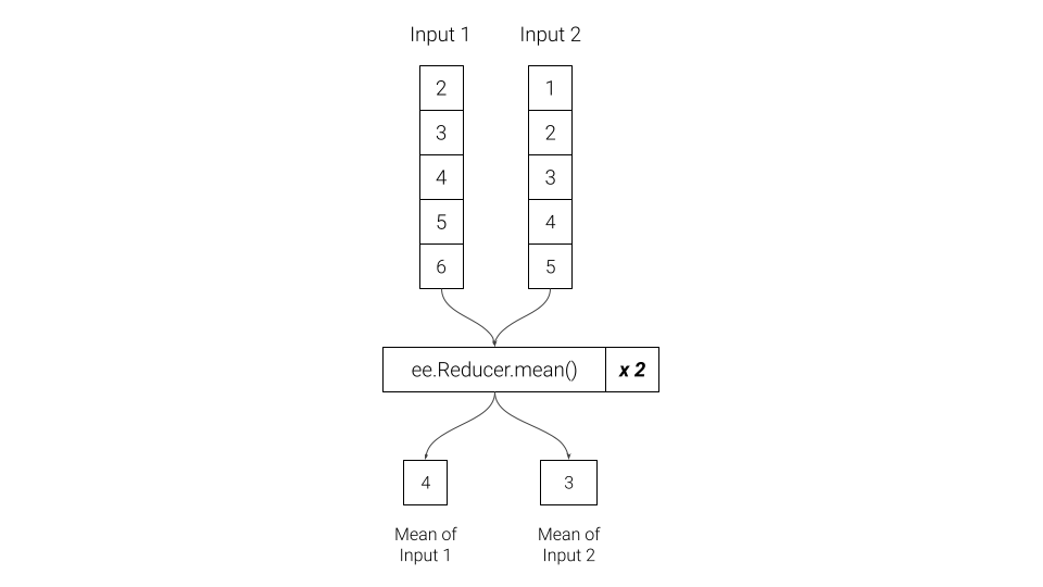
print('NDVI Statistics', stats);

02. Repeated Reducers

A reducer can be repeated multiple times to create a multi-input reducer. These are useful for computing the same statistics on different inputs.

Repeated Reducers

Open in Code Editor ↗

// Load the Ookla Speedtest Dataset
// https://gee-community-catalog.org/projects/speedtest/

var tiles = ee.FeatureCollection(
  'projects/sat-io/open-datasets/network/mobile_tiles/' +
  '2022-01-01_performance_mobile_tiles');

// Select a region
var admin2 = ee.FeatureCollection(
  'FAO/GAUL_SIMPLIFIED_500m/2015/level2');
var selected = admin2
  .filter(ee.Filter.eq('ADM0_NAME', 'India'))
  .filter(ee.Filter.eq('ADM2_NAME', 'Bangalore Urban'));
var geometry = selected.geometry();
Map.centerObject(geometry);

var filtered = tiles.filter(ee.Filter.bounds(geometry));
Map.addLayer(filtered, {color: 'blue'}, 'Broadband Speeds');

print(filtered.first());

// Let's compute average download speed
var stats = filtered.aggregate_mean('avg_d_kbps');
print('Average Download Speed (Mbps)', stats.divide(1000));

// If we want to compute stats on multiple properties
// we can use reducecolumns()

// Let's compute average download and upload speeds
var properties = ['avg_d_kbps', 'avg_u_kbps'];
// Since we have 2 properties, we need to repeat the reducer

var stats = filtered.reduceColumns({
  reducer: ee.Reducer.mean().repeat(2),
  selectors: properties});
print(stats.get('mean'));

// Extract and convert
var speeds = ee.List(stats.get('mean'));
print('Average Download Speed (Mbps)', speeds.getNumber(0).divide(1000));
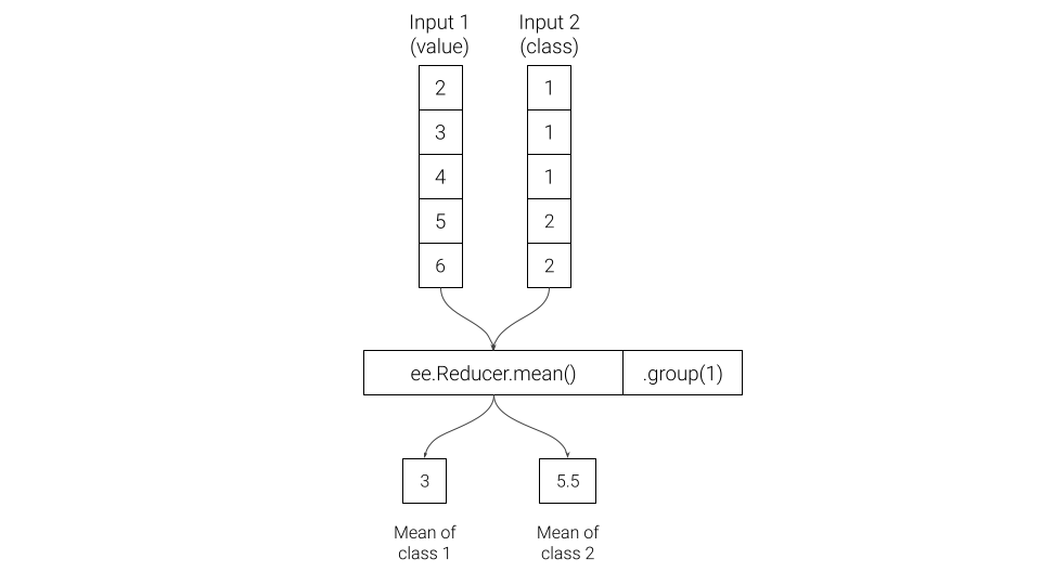
print('Average Upload Speed (Mbps)', speeds.getNumber(1).divide(1000));

03. Grouped Reducers

You can group the output of a reducer by the value of a specified input. These are useful in computing grouped statistics (i.e. statistics by category).

Grouped Reducers

Open in Code Editor ↗

// Select a region
var point = ee.Geometry.Point([77.6045, 12.8992]);
var bufferDistance = 5000;
var geometry = point.buffer(bufferDistance);
Map.centerObject(geometry, 12);
Map.addLayer(geometry, {color: 'gray'}, 'Buffer Zone');

var s2 = ee.ImageCollection('COPERNICUS/S2_SR');

// Write a function for Cloud masking
var maskS2clouds = function(image) {
  var qa = image.select('QA60')
  var cloudBitMask = 1 << 10;
  var cirrusBitMask = 1 << 11;
  var mask = qa.bitwiseAnd(cloudBitMask).eq(0).and(
             qa.bitwiseAnd(cirrusBitMask).eq(0))
  return image.updateMask(mask)
      .select('B.*')
      .copyProperties(image, ['system:time_start'])
}

// Write a function to scale the bands
var scaleImage = function(image) {
  return image
    .multiply(0.0001)
    .copyProperties(image, ['system:time_start'])
}

var filtered = s2
  .filter(ee.Filter.lt('CLOUDY_PIXEL_PERCENTAGE', 30))
  .filter(ee.Filter.bounds(geometry))
  .filter(ee.Filter.date('2021-01-01', '2022-01-01'))
  .map(maskS2clouds)
  .map(scaleImage);
  
// Create a median composite for 2021
var composite =  filtered.median();

var rgbVis = {min: 0.0, max: 0.3, bands: ['B4', 'B3', 'B2']};
Map.addLayer(composite.clip(geometry), rgbVis, '2020 Composite');

// We use the ESA WorldCover 2021 dataset
var worldcover = ee.ImageCollection('ESA/WorldCover/v200').first();

// The image has 11 classes
// Remap the class values to have continuous values
// from 0 to 10
var classified = worldcover.remap(
  [10, 20, 30, 40, 50, 60, 70, 80, 90, 95, 100],
  [0,  1 , 2,  3,  4,  5,  6,  7,  8,  9,  10]).rename('classification');

// Define a list of class names
var worldCoverClassNames= [
  'Tree Cover', 'Shrubland', 'Grassland', 'Cropland', 'Built-up',
  'Bare / sparse Vegetation', 'Snow and Ice', 
  'Permanent Water Bodies', 'Herbaceous Wetland', 
  'Mangroves', 'Moss and Lichen'];
// Define a list of class colors
var worldCoverPalette = [
  '006400', 'ffbb22', 'ffff4c', 'f096ff', 'fa0000',
  'b4b4b4', 'f0f0f0', '0064c8', '0096a0', '00cf75',
  'fae6a0'];
// We define a dictionary with class names
var classNames = ee.Dictionary.fromLists(
  ['0','1','2','3','4','5','6','7','8','9', '10'],
  worldCoverClassNames
);
// We define a dictionary with class colors
var classColors = ee.Dictionary.fromLists(
  ['0','1','2','3','4','5','6','7','8','9', '10'],
  worldCoverPalette
);
var worldCoverVisParams = {min:0, max:10, palette: worldCoverPalette};
Map.addLayer(classified.clip(geometry), worldCoverVisParams, 'Landcover');

var samples = composite.addBands(classified)
  .stratifiedSample({
    numPoints: 20,
    classBand: 'classification',
    region: geometry, 
    scale: 10,
    tileScale: 16
});
  
print('Stratified Samples', samples)

// We want to get average spectral value for a band
// grouped by class
var properties = ['B5', 'classification']
var stats = samples.reduceColumns({
    selectors: properties,
    reducer: ee.Reducer.mean().group({
      groupField: 1}),
});
var groupStats = ee.List(stats.get('groups'));
print(groupStats);

// Let's get average spectral value for every band
var bands = composite.bandNames();
var properties = bands.add('classification');

// Now we have multiple columns, so we have to repeat the reducer
var numBands = bands.length();

// We need the index of the group band
var groupIndex = properties.indexOf('classification');

var stats = samples.reduceColumns({
    selectors: properties,
    reducer: ee.Reducer.mean().repeat(numBands).group({
      groupField: groupIndex}),
});
var groupStats = ee.List(stats.get('groups'));
print(groupStats);

// We do some post-processing to format the results

var fc = ee.FeatureCollection(groupStats.map(function(item) {
  // Extract the means
  var values = ee.Dictionary(item).get('mean')
  var groupNumber = ee.Dictionary(item).get('group')
  var properties = ee.Dictionary.fromLists(bands, values)
  var withClass = properties.set('class', classNames.get(groupNumber))
  return ee.Feature(null, withClass)
}))
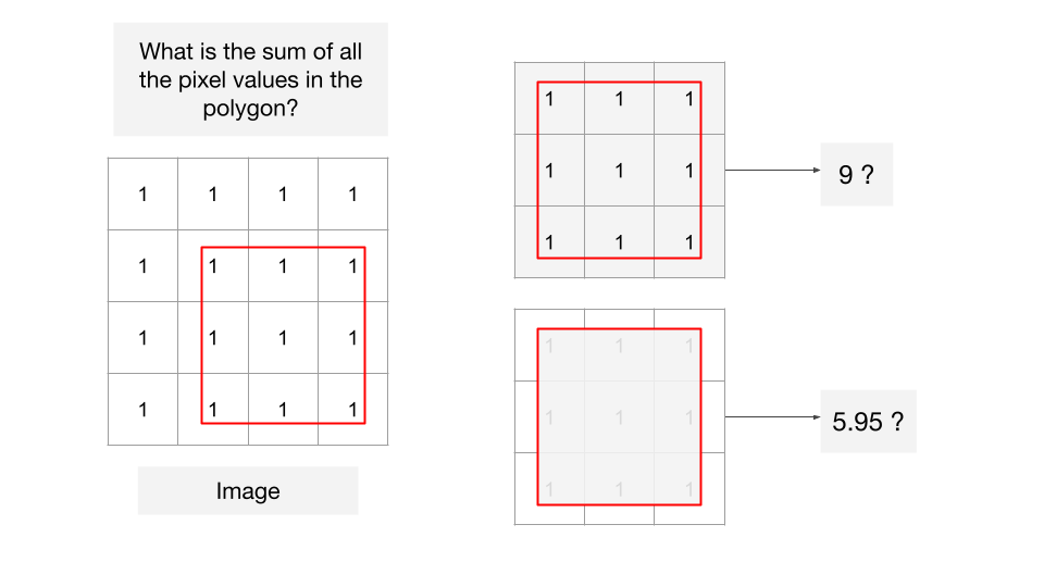
print('Average Spectral Value for Each Class', fc)

04. Weighted vs. Unweighted Reducers

Default calculations in Earth Engine uses weighted reducers. Weighted reducers account for fractional area of each pixel covered by the geometry. Unweighted reducers count pixels as whole if their centroid is covered by the geometry. You can choose to run any reducer in un-weighted mode using .unweighted(). Most software packages for remote sensing do not have support for weighted reducers, so Earth Engine users may choose to run their analysis un-weighted mode to verify and compare their results generated from other packages.

Weighted vs. Unweighted Reducers

Open in Code Editor ↗

// Example script demonstrating the different between
// weighted and un-weighted reducers in Earth Engine

// We are using a 4x4 pixel test image having each pixel
// value set to 1.
// with 1km pixels in EPSG:32643
// Code for generating such images is at 
// https://github.com/spatialthoughts/python-tutorials/blob/main/raster_from_array.ipynb
var image = ee.Image('users/ujavalgandhi/public/test_image_ones');
var pixels = ee.FeatureCollection('users/ujavalgandhi/public/test_image_pixels');
var test_geometry = ee.FeatureCollection('users/ujavalgandhi/public/test_geometry');
    
var visParams = {min:1, max:1, palette: ['white']};
Map.addLayer(image, visParams, 'Test Image');
Map.centerObject(image);

Map.addLayer(pixels, {color: 'black'}, 'Pixel Boundaries');

var centroids = image.sample({
  scale: 1000,
  region: image.geometry(),
  geometries: true
});
Map.addLayer(centroids, {color: 'cyan'}, 'Pixel Centroids');

var geometry = test_geometry.geometry();
Map.addLayer(geometry, {color: 'red'}, 'Region');

// 3rd party package for labelling
var style = require('users/gena/packages:style');
var textProperties = { textColor: 'ffffff', fontSize: 12, outlineColor: '000000'};
var labels = style.Feature.label(centroids, 'b1', textProperties);

Map.addLayer(labels, {}, 'labels');

// Weighted reducers account for fractional area of 
// each pixel covered by the geometry
var stats = image.reduceRegion({
  reducer: ee.Reducer.sum(),
  geometry: geometry,
  scale: 1000,
})
print('Sum of Pixels in Polygon (Weighted)', stats.get('b1'));

// Unweighted reducers count pixels as whole if their
// centroid is covered by the geometry
var stats = image.reduceRegion({
  reducer: ee.Reducer.sum().unweighted(),
  geometry: geometry,
  scale: 1000,
})
print('Sum of Pixels in Polygon (Un-weighted)', stats.get('b1'));

05. Zonal Statistics - Vector

Open in Code Editor ↗

// Vector Zonal Statistics

// We want to comptue the mean annual temperature
// for each ecoregion and each biome within a realm

// We use the EcoRegions FeatureCollection
var ecoregions = ee.FeatureCollection('RESOLVE/ECOREGIONS/2017');

// The dataset contains multiple polygons for each ecoregion
// The layer contains polygons for -> 846 Ecoregions
// Ecoregions are grouped into -> 14 Biomes
// Biomes are groouped into -> 8 Realms
print(ecoregions.aggregate_array('REALM').distinct());

// Let's filter to ecoregions in a realm
var realm = 'Australasia';
var filtered = ecoregions.filter(ee.Filter.eq('REALM', realm));

// We use the WorldClim V1 dataset that contains
// historical climate data from 1960-1990
var worldclim = ee.Image('WORLDCLIM/V1/BIO');

// Select 'annual mean temperature' band
// and apply scaling factor
var temperature = worldclim.select('bio01').multiply(0.1);

// Visualize Temperature and Ecoregions
var palette = ['#4575b4', '#91bfdb', '#e0f3f8', 
  '#ffffbf', '#fee090', '#fc8d59', '#d73027']
Map.addLayer(temperature, {min:10, max:25, palette: palette},
  'Annual Mean Temparature')
Map.addLayer(filtered.filter(ee.Filter.eq('REALM', realm)), {color: 'blue'}, 'Ecoregions');

// Calculate Average Annual Mean Temperature per Ecoregion

// Get the native resolution of the image
var scale = worldclim.projection().nominalScale()

var zonalStats = temperature.reduceRegions({
  collection: filtered,
  reducer: ee.Reducer.mean().setOutputs(['meantemp']),
  scale: scale})

// Output of reduceRegions() is a FeatureCollection
print('Ecoregions with Mean Temp', zonalStats.first());

// We have 1 polygon per ecoregion with its mean temperature
// Group them by biome and compute mean temperature per biome
var zonalGroupStats = zonalStats.reduceColumns({
  reducer: ee.Reducer.mean().setOutputs(['meantemp'])
    .group({groupField: 1, groupName: 'biome'}),
  selectors: ['meantemp', 'BIOME_NAME']})

print('Biomes with Mean Temp', zonalGroupStats);

// Process the results
var groups = ee.List(zonalGroupStats.get('groups'));

var results = groups.map(function(item) {
  // Extract the mean
  var meanTemp = ee.Dictionary(item).get('meantemp');
  // The group name is what we specified in the grouped reducer
  var biomeName = ee.Dictionary(item).get('biome');
  return ee.Feature(null, {
    'BIOME_NAME': biomeName,
    'meantemp': meanTemp});
});

var zonalGroupStatsFc = ee.FeatureCollection(results);
print('Biomes with Mean Temp (Processed)', zonalGroupStatsFc);

// Export the results
Export.table.toDrive({
  collection: zonalStats,
  description: 'Mean_Temp_By_Ecoregion',
  folder: 'earthengine',
  fileNamePrefix: 'mean_temp_by_ecoregion',
  fileFormat: 'CSV',
  selectors: ['BIOME_NAME', 'ECO_NAME', 'meantemp']
})

Export.table.toDrive({
  collection: zonalGroupStatsFc,
  description: 'Mean_Temp_By_Biome',
  folder: 'earthengine',
  fileNamePrefix: 'mean_temp_by_biome',
  fileFormat: 'CSV',
  selectors: ['BIOME_NAME', 'meantemp']
})

06. Zonal Statistics - Raster

Open in Code Editor ↗

// Raster Zonal Statistics

// We want to use unsupervised classification on a source image
// and automatically detect water cluster by picking the cluster
// with highest MNDWI value.

// Create a composite for the selected region
var admin2 = ee.FeatureCollection("FAO/GAUL_SIMPLIFIED_500m/2015/level2");
var s2 = ee.ImageCollection("COPERNICUS/S2_SR_HARMONIZED");

var selected = admin2.filter(ee.Filter.eq('ADM2_NAME', 'Bangalore Urban'))
var geometry = selected.geometry()

// Cloud masking function
function maskS2clouds(image) {
  var qa = image.select('QA60')
  // Bits 10 and 11 are clouds and cirrus, respectively.
  var cloudBitMask = 1 << 10;
  var cirrusBitMask = 1 << 11;
  // Both flags should be set to zero, indicating clear conditions.
  var mask = qa.bitwiseAnd(cloudBitMask).eq(0).and(
             qa.bitwiseAnd(cirrusBitMask).eq(0))
  // Return the masked and scaled data, without the QA bands.
  return image.updateMask(mask).divide(10000)
      .select('B.*')
      .copyProperties(image, ['system:time_start'])
}

var filtered = s2.filter(ee.Filter.lt('CLOUDY_PIXEL_PERCENTAGE', 30))
  .filter(ee.Filter.date('2019-01-01', '2020-01-01'))
  .filter(ee.Filter.bounds(geometry))
  .map(maskS2clouds);
  
var image = filtered.median().clip(geometry); 


// Calculate  Normalized Difference Vegetation Index (NDWI)
// 'GREEN' (B3) and 'NIR' (B8)
var ndwi = image.normalizedDifference(['B3', 'B8']).rename(['ndwi']);
 
// Calculate Modified Normalized Difference Water Index (MNDWI)
// 'GREEN' (B3) and 'SWIR1' (B11)
var mndwi = image.normalizedDifference(['B3', 'B11']).rename(['mndwi']); 

// Select the MIR (SWIR2) band (B12)
var mir2 = image.select('B12').multiply(0.0001).rename('mir2')

var stackedImage = ndwi.addBands(mndwi).addBands(mir2)

// Make the training dataset for unsupervised clustering
var training = stackedImage.sample({
  region: geometry,
  scale: 10,
  numPixels: 1000
});
print(training.first())

// Instantiate the clusterer and train it.
var clusterer = ee.Clusterer.wekaCascadeKMeans({
  minClusters: 2,
  maxClusters: 10}).train(training);

// Cluster the stacked image
var clustered = stackedImage.cluster(clusterer);

// Visualize the results
Map.setCenter(77.61, 13.08, 14)

Map.centerObject(geometry, 10);
var rgbVis = {min: 0.0, max: 0.3, bands: ['B4', 'B3', 'B2']};
Map.addLayer(image, rgbVis, 'Image');
Map.addLayer(clustered.randomVisualizer(), {}, 'clusters')

// We need to identify which of the clusters represent water
// We use the MNDWI band and select the cluster with the 
// highest average MNDWI values of all pixels within the cluster

// Calculate the stats on MNDWI band, grouped by clusters
var stats = mndwi.addBands(clustered).reduceRegion({
  reducer: ee.Reducer.mean().group({
    groupField: 1,
    groupName: 'cluster',
  }),
  geometry: geometry,
  scale: 100, // Approximate stats
  maxPixels: 1e8
});
print(stats)

// Extract the cluster-wise stats as a list of lists
// We get a list in the following format
// [[avg_mndwi, cluster_number], [avg_mndwi, cluster_number] ...]]
var groupStats = ee.List(stats.get('groups'))

var groupStatsLists = groupStats.map(function(item) {
      var areaDict = ee.Dictionary(item)
      var clusterNumber = ee.Number(
        areaDict.get('cluster'))
      var mndwi = ee.Number(
        areaDict.get('mean'))
      return ee.List([mndwi, clusterNumber])
    })
    
// Use the ee.Reducer.max() on the list of lists
// It will pick the list with the highest MNDWI
var waterClusterList = ee.Dictionary(ee.List(groupStatsLists).reduce(ee.Reducer.max(2)))

// Extract the cluster number
var waterCluster = ee.Number(waterClusterList.get('max1'))

// Select all pixels from the water cluster and mask everything else
var water = clustered.eq(waterCluster).selfMask()

var waterVis = {min:0, max:1, palette: ['white', 'blue']}
Map.addLayer(water, waterVis, 'water')

// Interactive visualization may time-out for large images
// Export the image to use the batch processing mode
Export.image.toDrive({
  image: water,
  description: 'Water_Cluster',
  folder: 'earthengine',
  fileNamePrefix: 'water_cluster',
  region: geometry,
  scale: 20,
  maxPixels: 1e10})

Joins

Coming Soon…

Regressions

Coming Soon…

Vector Data Processing and Visualization

Coming Soon…

License

The course material (text, images, presentation, videos) is licensed under a Creative Commons Attribution 4.0 International License.

The code (scripts, Jupyter notebooks) is licensed under the MIT License. For a copy, see https://opensource.org/licenses/MIT

You are free to re-use and adapt the material but are required to give appropriate credit to the original author as below:

Citing and Referencing

You can cite the course materials as follows

Gandhi, Ujaval, 2023. Advanced Concepts in Google Earth Engine course. Spatial Thoughts. https://courses.spatialthoughts.com/gee-advanced.html

Advanced Concepts in Google Earth Engine (Full Course Material)

A Deep-dive into Reducers, Joins, Regressions and Vector Data Processing in GEE.

Ujaval Gandhi

Introduction

Get the Course Materials

1. Reducers

01. Combined Reducers

02. Repeated Reducers

03. Grouped Reducers

04. Weighted vs. Unweighted Reducers

05. Zonal Statistics - Vector

06. Zonal Statistics - Raster

Joins

Regressions

Vector Data Processing and Visualization

License

Citing and Referencing

Advanced Concepts in Google Earth Engine (Full Course Material)

A Deep-dive into Reducers, Joins, Regressions and Vector Data Processing in GEE.

Ujaval Gandhi

Introduction

Sign-up for Google Earth Engine

Get the Course Materials

1. Reducers

01. Combined Reducers

02. Repeated Reducers

03. Grouped Reducers

04. Weighted vs. Unweighted Reducers

05. Zonal Statistics - Vector

06. Zonal Statistics - Raster

Joins

Regressions

Vector Data Processing and Visualization

License

Citing and Referencing