Introduction

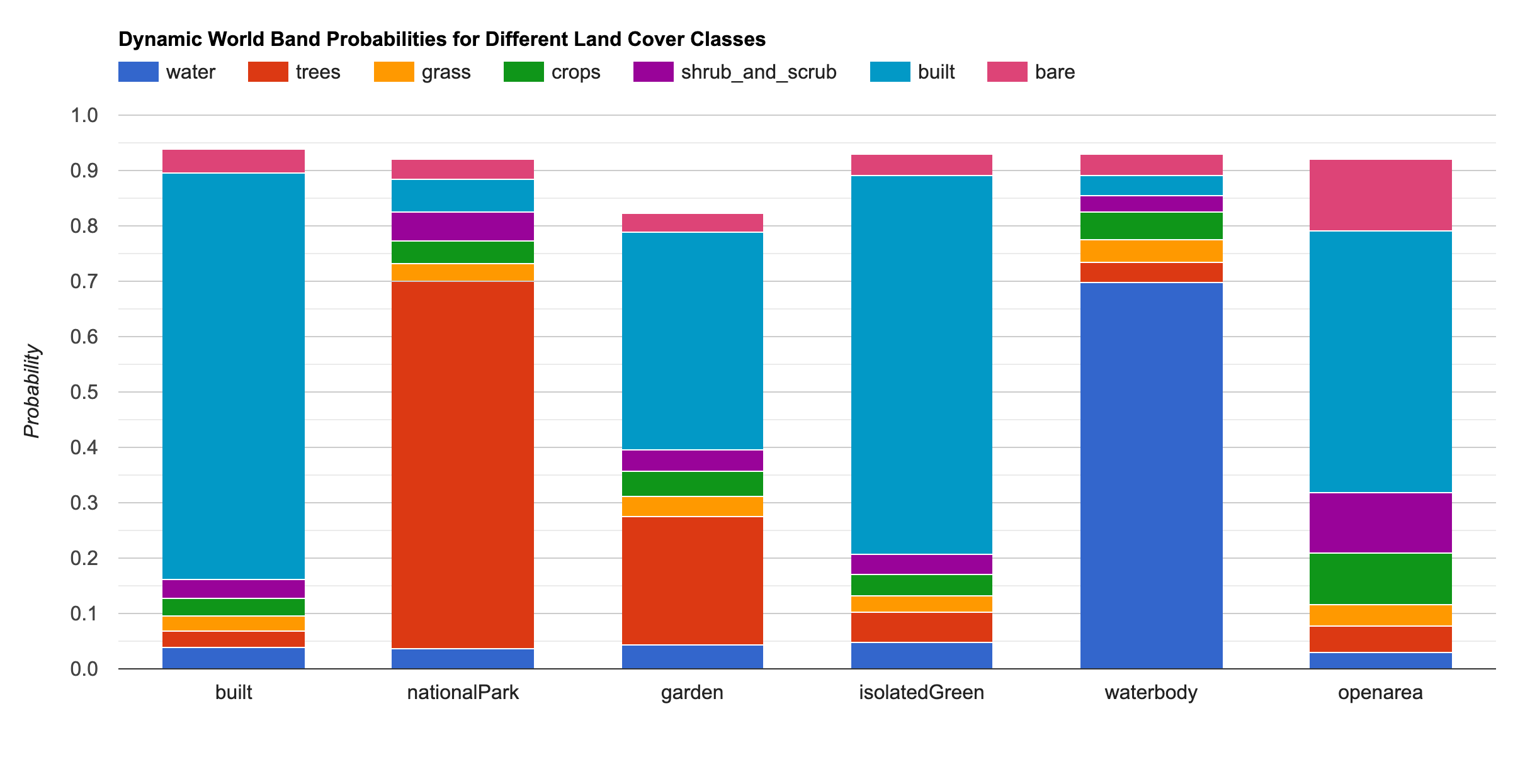
Dynamic World is a landcover product developed by Google and World Resources Institute (WRI). It is a unique dataset that is designed to make it easy for users to do near real-time monitoring of landcover changes. The Dynamic World (DW) model gives you the the probability of the pixel belonging to each of the 9 different landcover classes and the dataset is updated continuously with detections from new Sentinel-2 scenes as soon as they are available. This makes DW ideal for change detection and monitoring applications. This workshop covers a wide range of examples for using Dynamic World dataset in Google Earth Engine (GEE) for landcover monitoring.

View the Presentation ↗

Quiz - Introduction to Dynamic World

This is a short quiz to test your understanding of the Dynamic World dataset.

Launch Quiz ↗.

Setting up the Environment

Get the Workshop Materials

The workshop material and exercises are in the form of Earth Engine scripts shared via a code repository.

Click this link to open Google Earth Engine code editor and add the repository to your account.
If successful, you will have a new repository named users/ujavalgandhi/GEE-DW-Monitoring in the Scripts tab in the Reader section.
Verify that your code editor looks like below

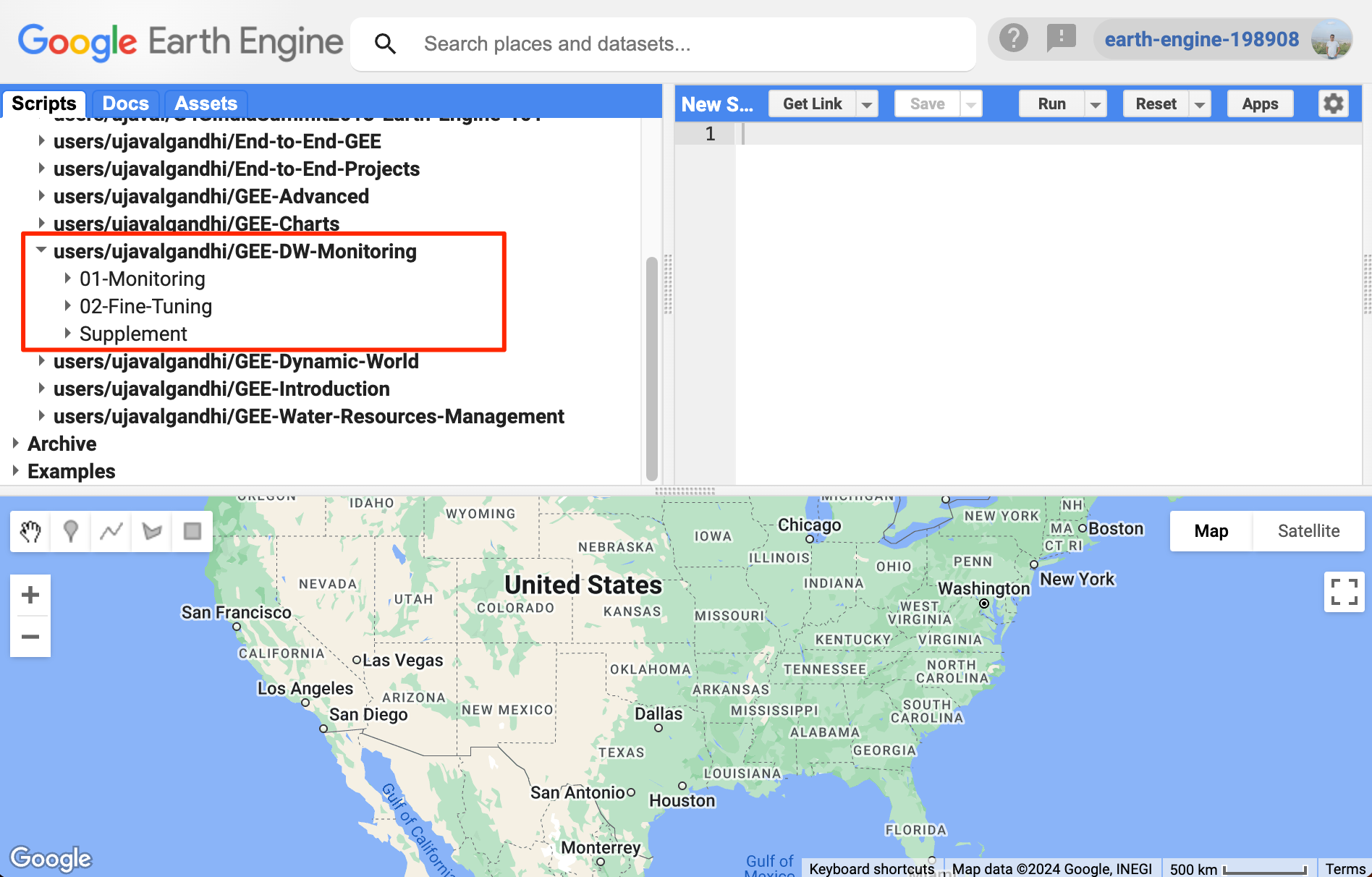
Code Editor After Adding the Workshop Repository

If you do not see the repository in the Reader section, click Refresh repository cache button in your Scripts tab and it will show up.

Module 1: Monitoring Landcover Changes

01. Monitoring Surface Water

Surface Water Extent Monitoring for KrishnaRajaSagara Reservoir, India

Open in Code Editor ↗

// **************************************************************
// Monitoring Surface Water with Dynamic World

// This script shows how to use Dynamic World 'water' probability
// band to select a threshold and extract water pixels
// for the chosen region and calculate surface water area

// The script selects all Dynamic World images with no cloud cover
// within the region to ensure the calculated area is consistent.
// **************************************************************

// Choose a region
var geometry = ee.Geometry.Polygon([[
  [76.37422, 12.5721],
  [76.37422, 12.3736],
  [76.62073, 12.3736],
  [76.62073, 12.5721]]
]);
// Delete the 'geometry' variable and draw a polygon
// over a waterbody
Map.centerObject(geometry);
// Choose a time period
var startDate = ee.Date.fromYMD(2023, 1, 1);
var endDate = startDate.advance(1, 'year');

// Visualize the Dynamic World images
// for the chosen region and time period

var probabilityBands = [
  'water', 'trees', 'grass', 'flooded_vegetation', 'crops',
  'shrub_and_scrub', 'built', 'bare', 'snow_and_ice'
];

// Filter the Dynamic World collection
var dwFiltered = ee.ImageCollection('GOOGLE/DYNAMICWORLD/V1')
  .filter(ee.Filter.date(startDate, endDate))
  .filter(ee.Filter.bounds(geometry))
  .select(probabilityBands);

// Function that adds a property to each image
// with the percentage of cloud-free pixels in the
// chosen geometry
var calculateCloudCover = function(image) {
  // The Dynamic World images have some pixels
  // that are masked.
  // We count the number of unmasked pixels
  // Select any band, since all bands have the same mask
  // Working with a single band makes the analysis simpler
  var bandName = 'water';
  var band = image.select(bandName);
  var withMaskStats = band.reduceRegion({
    reducer: ee.Reducer.count(),
    geometry: geometry,
    scale: 100,
    bestEffort: true
  });
  var cloudFreePixels = withMaskStats.getNumber(bandName);
  
  // Remove the mask and count all pixels
  var withoutMaskStats = band.unmask(0).reduceRegion({
    reducer: ee.Reducer.count(),
    geometry: geometry,
    scale: 100,
    bestEffort: true
  });
  
  var totalPixels = withoutMaskStats.getNumber(bandName);
  
  var cloudCoverPercentage = ee.Number.expression(
    '100*(totalPixels-cloudFreePixels)/totalPixels', {
      totalPixels: totalPixels,
      cloudFreePixels: cloudFreePixels
    });
  
  // Add a 'date' property for ease of selection  
  var dateString = ee.Date(image.date()).format('YYYY-MM-dd');

  return image.set({
    'CLOUDY_PIXEL_PERCENTAGE_REGION': cloudCoverPercentage,
    'date': dateString
  });
};

var dwFilteredWithCount = dwFiltered.map(calculateCloudCover);

print(dwFilteredWithCount.first());

// Filter using the newly created property
var dwImages = dwFilteredWithCount
  .filter(ee.Filter.lt('CLOUDY_PIXEL_PERCENTAGE_REGION', 1));
print('Cloud Free Images in Region', dwImages.size());


var s2 = ee.ImageCollection('COPERNICUS/S2_HARMONIZED');

var s2Bands = s2.first().select('B.*').bandNames();
var images = dwImages.linkCollection(s2, s2Bands);

var getWater = function(image) {
  // Select a threshold for water probability
  var waterThreshold = 0.4;
  // Select all pixels where 
  // 'water' probability > waterThreshold
  var water = image.select('water').gt(waterThreshold);
  return water.selfMask();
};


// Display the image with the given ID.
var display = function(date) {
  var layers = Map.layers();
  layers.forEach(function(layer) {
    layer.setShown(false);
  });
  
  var image = images.filter(ee.Filter.eq('date', date)).mosaic();
  var cloudMask = image.select('water').mask();
  var rgbVis = {min:0, max:2500, gamma: 1.2, bands: ['B4', 'B3', 'B2']};
  var falseColorVis = {min:0, max:2500, gamma: 1.2, bands: ['B12', 'B8', 'B4']};
  var s2Vis = rgbVis;
  Map.addLayer(image.updateMask(cloudMask), s2Vis, 'Image_' + date);
  
  var probabilityVis = {min:0, max:1, bands: ['water'],
    palette: ['#8c510a','#d8b365','#f6e8c3','#c7eae5','#5ab4ac','#01665e']};
  
  Map.addLayer(image, probabilityVis, 'Water Probability_' + date);
  
  var water = getWater(image);

  var waterVis = {min:0, max:1, palette: ['white', 'blue']};
  
  var region = ee.FeatureCollection([ee.Feature(geometry)]);
  var border = ee.Image().byte().paint(region, 1, 1);
  Map.addLayer(border, {}, 'Selected Region');
  
  Map.addLayer(water.clip(geometry), waterVis, 'Water_' + date, false);
  
  // Calculate Surface Water Area
  var area = water.multiply(ee.Image.pixelArea()).reduceRegion({
    reducer: ee.Reducer.sum(),
    geometry: geometry,
    scale: 10,
    maxPixels: 1e10,
    tileScale: 16
  });
  var waterArea = area.getNumber('water').divide(1e6).format('%.2f');
  print('Surface Water Area (Sq.Km.) ' + date, waterArea);
};

// Get the list of IDs and put them into a select
images.aggregate_array('date').distinct().evaluate(function(ids) {
  var selector = ui.Select({
    items: ids,
    onChange: display,
  });
  Map.add(selector);
  selector.setValue(ids[0], true);
});

02. Monitoring Urban Growth

Urban Changes in São Paulo

Open in Code Editor ↗

// **************************************************************
// Monitoring Urban Growth with Dynamic World

// This script shows how to track changes in built environment 
// using the 'built' probability band of Dynamic World dataset

// It selects all pixels with large changes in 'built' probability
// over the selected time period.
// **************************************************************

// Choose a region
var geometry = ee.Geometry.Polygon([[
  [-46.95235487694674, -23.325163502957597],
  [-46.95235487694674, -23.83113543079588],
  [-46.29592177147799, -23.83113543079588],
  [-46.29592177147799, -23.325163502957597]
]]);
          
// Delete the 'geometry' variable and draw a polygon
// over a waterbody
Map.centerObject(geometry, 10);

// Define the before and after time periods.
var beforeYear = 2017;
var afterYear = 2023;

// Create start and end dates for the before and after periods.
var beforeStart = ee.Date.fromYMD(beforeYear, 1 , 1);
var beforeEnd = beforeStart.advance(1, 'year');

var afterStart = ee.Date.fromYMD(afterYear, 1 , 1);
var afterEnd = afterStart.advance(1, 'year');

// Load the Dynamic World collection
var dw = ee.ImageCollection('GOOGLE/DYNAMICWORLD/V1')

// Filter the collection and select the 'built' band.
var dwFiltered = dw
  .filter(ee.Filter.bounds(geometry))
  .select('built');

// Create mean composites
var beforeDw = dwFiltered.filter(
  ee.Filter.date(beforeStart, beforeEnd)).mean();
  
var afterDw = dwFiltered.filter(
  ee.Filter.date(afterStart, afterEnd)).mean();


// Add Sentinel-2 Composites to verify the results.
var s2 = ee.ImageCollection('COPERNICUS/S2_HARMONIZED')
     .filterBounds(geometry)
     .filter(ee.Filter.lt('CLOUDY_PIXEL_PERCENTAGE', 35));

// Create a median composite from sentinel-2 images.
var beforeS2 = s2.filterDate(beforeStart, beforeEnd).median();
var afterS2 = s2.filterDate(afterStart, afterEnd).median();
  
// Visualize images
var s2VisParams = {bands: ['B4', 'B3', 'B2'], min: 0, max: 3000};
Map.addLayer(beforeS2.clip(geometry), s2VisParams, 'Before S2');
Map.addLayer(afterS2.clip(geometry), s2VisParams, 'After S2');

// **************************************************************
// Find Change Pixels
// **************************************************************

// Select all pixels that have experienced large change
// in 'built' probbility
var builtChangeThreshold = 0.3; 
var newUrban = afterDw.subtract(beforeDw).gt(builtChangeThreshold);


// **************************************************************
// Visualize 
// **************************************************************

// Mask all pixels with 0 value using selfMask()
var newUrbanMasked = newUrban.selfMask();

var changeVisParams = {min: 0, max: 1, palette: ['white', 'red']};
Map.addLayer(
  newUrbanMasked.clip(geometry), changeVisParams, 'New Urban Areas');

03. Monitoring Deforestation

Deforestation Monitoring in Brazil

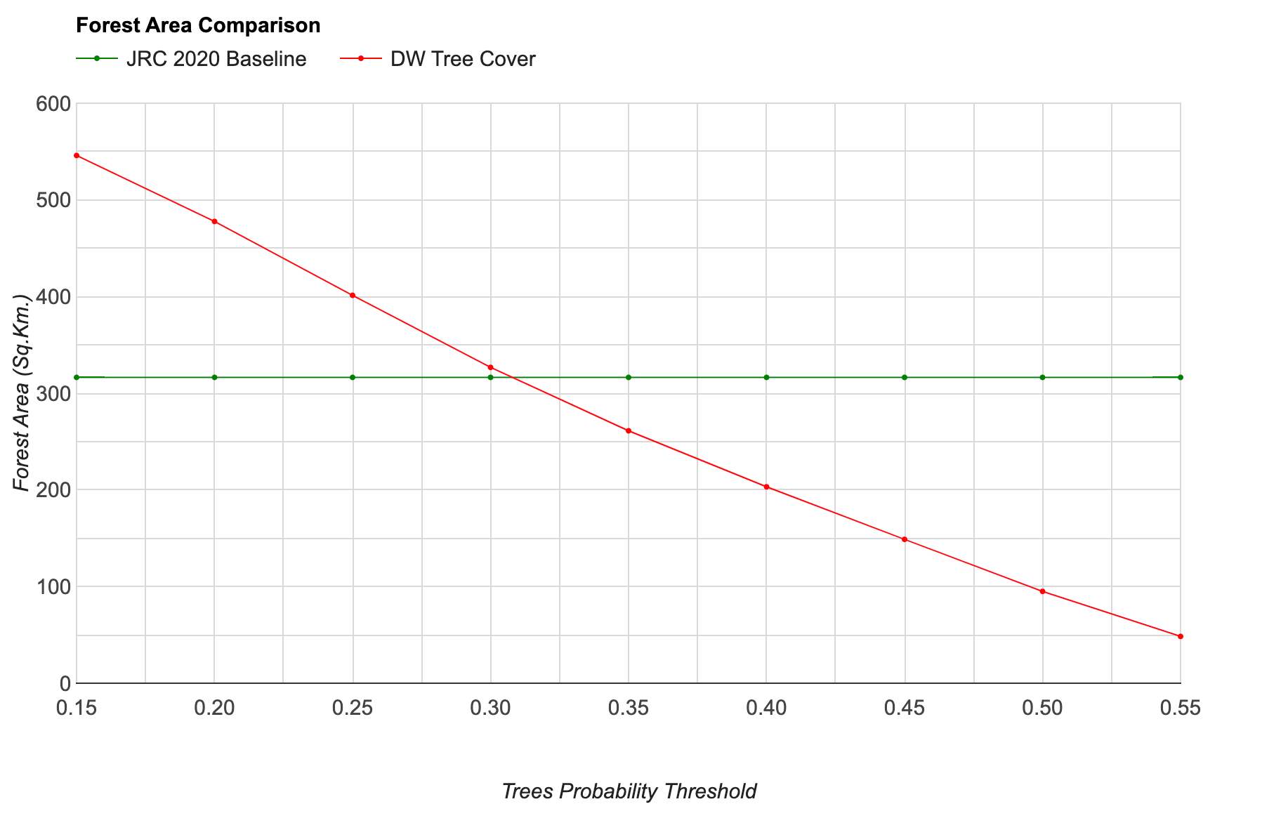
Discovering Optimal Probability Threshold

Open in Code Editor ↗

// ================================================================
// Monitoring Deforestation using Dynamic World

// This script shows how to use Dynamic World 'trees' probability band
// to identify forest pixels and calculate loss of forest
// between the chosen years.

// To calibrate the threshold for the selected region, we use the
// EC JRC Forest cover baseline 2020 dataset and determine
// the appropriate threshold for the 'trees' probability
// by comparing the forest area from both the JRC and DW datasets
// and picking the threshold with the closest match.

// Finally the change detection output is masked using the JRC
// dataset to detect areas deforested since the EC JRC Forest
// cover baseline 2020.

// This script adapted from the original example by
// created by Hugh Lynch from Google
// ================================================================

// Choose a region
// Delete the 'geometry' variable and draw a polygon
var geometry = ee.Geometry.Polygon([[
  [-41.014524684034946, -5.710627921629724],
  [-41.014524684034946, -5.880045590317402],
  [-40.70278762348807, -5.880045590317402],
  [-40.70278762348807, -5.710627921629724]
]]);
          
var baselineYear = 2020;
var comparisonYear = 2023;

// Create start and end dates for the before and after periods.
var beforeStart = ee.Date.fromYMD(baselineYear, 1, 1);
var beforeEnd = beforeStart.advance(1, 'year');

var afterStart = ee.Date.fromYMD(comparisonYear, 1 , 1);
var afterEnd = afterStart.advance(1, 'year');

// Load the Dynamic World collection
var dw = ee.ImageCollection('GOOGLE/DYNAMICWORLD/V1');

// Filter the collection and select the 'built' band.
var dwFiltered = dw
  .filter(ee.Filter.bounds(geometry))
  .select('trees');

// Create mean composites
var beforeDw = dwFiltered.filter(
  ee.Filter.date(beforeStart, beforeEnd)).mean();
  
var afterDw = dwFiltered.filter(
  ee.Filter.date(afterStart, afterEnd)).mean();

// ================================================================
// Threshold Discovery
// ================================================================

// We do not know what is the appropriate threshold for
// the 'trees' probabity band that represents
// forest in the chosen region of interest

// We can try a range of thresholds a pick the one
// that has the best match with the baseline
var treesThresholds = ee.List.sequence(0.15, 0.55, 0.05);

// We compute the area of forest for each of threshold
// including undercount and overcount of forest pixels
// by comparing it with JRC baseline

// Add EC JRC global map of forest cover 2020
var jrcForest = ee.ImageCollection('JRC/GFC2020/V1').first();
// When zoomed out, the JRC Forest value remains 1, but the mask is fractional.
var jrcForestMask = jrcForest.mask().gt(0.5).rename('jrc_baseline');

var thresholdData = treesThresholds.map(function(treesThreshold) {
  var dwTrees = beforeDw.gt(ee.Number(treesThreshold)).rename('dw_trees');
  var areaImage = ee.Image.cat([dwTrees, jrcForestMask])
    .multiply(ee.Image.pixelArea())
    .divide(1e6);
  var stats = areaImage.reduceRegion({
    reducer: ee.Reducer.sum(),
    geometry: geometry,
    scale: 10,
    maxPixels: 1e10,
    tileScale: 16
  });

  var properties = stats.combine({
    'threshold': treesThreshold,
  });
  return ee.Feature(geometry, properties);
});

var thresholdFc = ee.FeatureCollection(thresholdData);

// Create a chart
var chart = ui.Chart.feature.byFeature({
  features: thresholdFc,
  xProperty: 'threshold',
  yProperties: ['jrc_baseline', 'dw_trees']
}).setChartType('LineChart')
  .setOptions({
    lineWidth: 1,
    pointSize: 2,
    title: 'Forest Area Comparison',
    vAxis: {
      title: 'Forest Area (Sq.Km.)',
      gridlines: {color:'#d9d9d9'},
      minorGridlines: {color:'#d9d9d9'}
    },
    hAxis: {
      title: 'Trees Probability Threshold',
      gridlines: {color:'#d9d9d9'},
      minorGridlines: {color:'#d9d9d9'}
    },
    series: {
      0: {color: 'green', labelInLegend: 'JRC 2020 Baseline'},
      1: {color: 'red', labelInLegend: 'DW Tree Cover'}
    },
    chartArea: {left:50, right:100},
    legend: {
      position: 'top'
    }

  })
;
print(chart);

// ================================================================
// Change Detection
// ================================================================

// Select a threshold for Forest
var treesThreshold = 0.3;
// Find all pixels that were 
// forest before and not forest after
var beforeForest = beforeDw.gt(treesThreshold);
var afterForest = afterDw.gt(treesThreshold);

var lostForest = beforeForest.and(afterForest.not());
// Mask pixels with small change
var treeProbabilityLoss = beforeDw.subtract(afterDw);
var noiseThreshold = 0.2;
var lostForestSignificant = lostForest
  .updateMask(treeProbabilityLoss.gt(noiseThreshold));

// Select only loss pixels that were classified
// as forest in the JRC 2020 baseline
// Add EC JRC global map of forest cover 2020
var jrcForest = ee.ImageCollection('JRC/GFC2020/V1').first();
// When zoomed out, the JRC Forest value remains 1, but the mask is fractional.
var jrcForestMask = jrcForest.mask().gt(0.5);
var lostForestAndJrc = lostForestSignificant.updateMask(jrcForestMask);

// ================================================================
// Visualization
// ================================================================

// Add Sentinel-2 Composites to verify the results.
var s2 = ee.ImageCollection("COPERNICUS/S2_SR_HARMONIZED");

var filtered = s2
  .filter(ee.Filter.bounds(geometry));

// Load the Cloud Score+ collection for cloud masking
var csPlus = ee.ImageCollection('GOOGLE/CLOUD_SCORE_PLUS/V1/S2_HARMONIZED');
var csPlusBands = csPlus.first().bandNames();

// We need to add Cloud Score + bands to each Sentinel-2
// image in the collection
// This is done using the linkCollection() function
var filteredS2WithCs = filtered.linkCollection(csPlus, csPlusBands);

// Function to mask pixels with low CS+ QA scores.
function maskLowQA(image) {
  var qaBand = 'cs';
  var clearThreshold = 0.5;
  var mask = image.select(qaBand).gte(clearThreshold);
  return image.updateMask(mask);
}

var filteredMasked = filteredS2WithCs
  .map(maskLowQA)
  .select('B.*');

var beforeS2 = filteredMasked
  .filter(ee.Filter.date(beforeStart, beforeEnd))
  .median();
var afterS2 = filteredMasked
  .filter(ee.Filter.date(afterStart, afterEnd))
  .median();

var s2Composite = filteredMasked.median();
var s2VisParams = {bands: ['B4', 'B3', 'B2'], min: 300, max: 1500, gamma: 1.2};

Map.centerObject(geometry);
Map.addLayer(beforeS2.clip(geometry), s2VisParams, 'Before S2 (Baseline)');
Map.addLayer(afterS2.clip(geometry), s2VisParams, 'After S2');
Map.addLayer(jrcForest.clip(geometry), {palette: ['4D9221']}, 'JRC Forest Cover 2020', false);
Map.addLayer(lostForestSignificant.clip(geometry), {palette: ['fa9fb5']}, 'Forest Loss', false);
Map.addLayer(lostForestAndJrc.clip(geometry), {palette: ['red']}, 'Forest Loss within JRC Baseline)');

04. Monitoring Restoration Trends

Restoration Monitoring in Maasai Mau Forest, Kenya

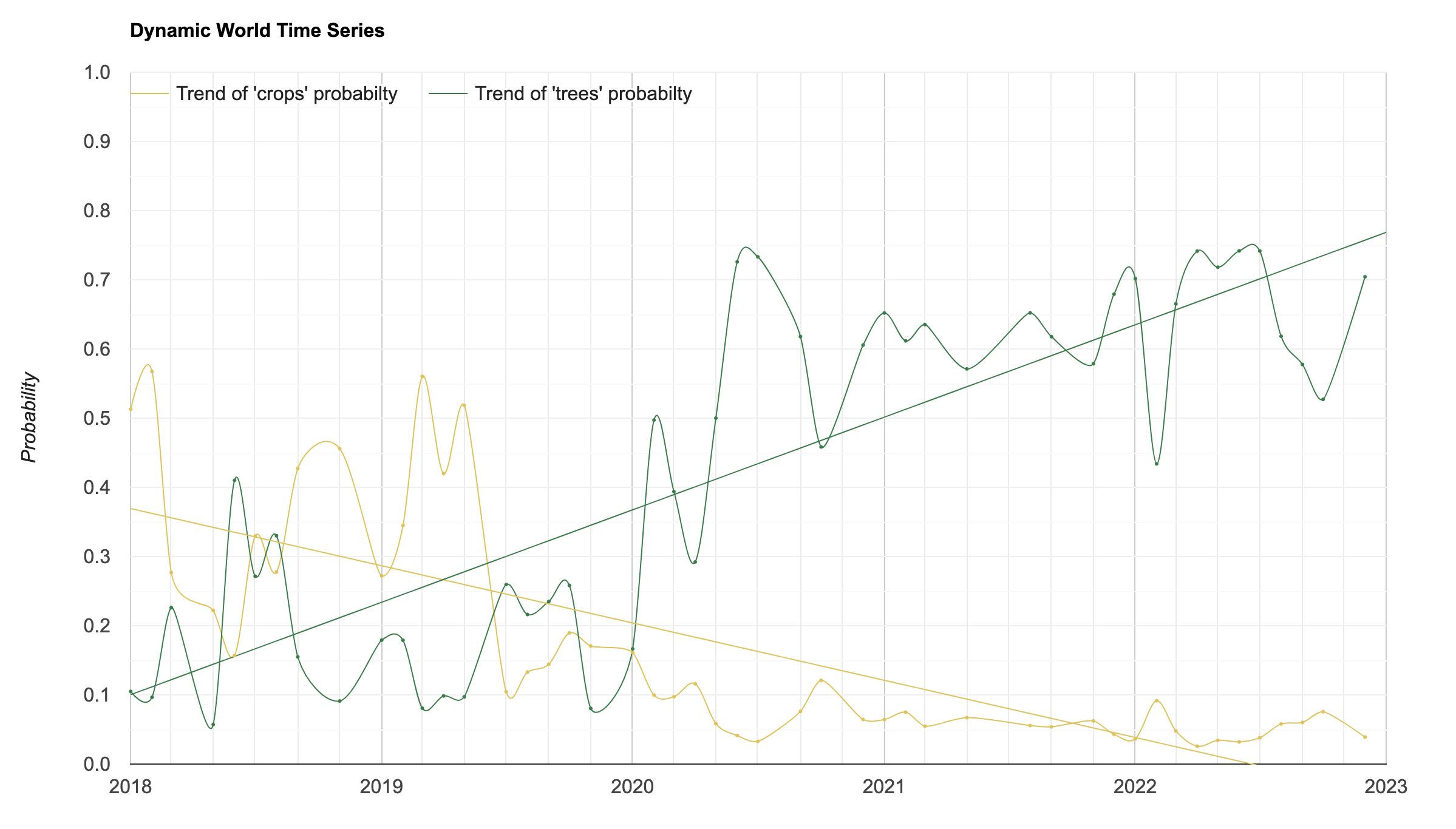
Trend of Landcover Probabilties

Open in Code Editor ↗

// **************************************************************
// Monitoring Restoration Trends using Dynamic World

// This script show how to analyse the trend of landcover change
// using a set of probability bands from Dynamic World

// This script first aggregates the Dynamic World images
// to monitor a forest restoration project in Maasai Mau Forest
// block in Kenya. Several interventions have helped restore 
// grassland and forest since 2019.

// The original time-series is quite noisy so we first aggregate
// it to a monthly mean probability time-series and compute a
// per-pixel trend using Sens Slope reducer.
// The resulting image is used to identify regions with positive
// trend of 'grass' and 'trees' probabilities.
// **************************************************************

// Use the Boundary of the Maasai Mau Forest Block as the geometry
var mmf = ee.FeatureCollection('users/ujavalgandhi/kenya/mmf');
var geometry = mmf.geometry();
Map.centerObject(geometry, 12);

// Define the time periods for trend analysis
var startYear = 2018;
var endYear = 2022;

var years = ee.List.sequence(startYear, endYear);
var months = ee.List.sequence(1, 12);

// Load the Dynamic World collection
var dw = ee.ImageCollection('GOOGLE/DYNAMICWORLD/V1')

var probabilityBands = [
  'water', 'trees', 'grass', 'flooded_vegetation', 'crops',
  'shrub_and_scrub', 'built', 'bare', 'snow_and_ice'
];

// Filter the collection and select the 'built' band.
var dwFiltered = dw
  .filter(ee.Filter.bounds(geometry))
  .select(probabilityBands);

// Create monthly mean images
var monthlyImages = years.map(function(year) {
  return months.map(function(month) {
    var filtered = dwFiltered
      .filter(ee.Filter.calendarRange(year, year, 'year'))
      .filter(ee.Filter.calendarRange(month, month, 'month'))
    var monthly = filtered.mean()
    return monthly.set({
      'month': month,
      'year': year,
      'system:time_start': ee.Date.fromYMD(year, month, 1).millis(),
      'num_images': filtered.size()
    });
  });
}).flatten();

// Create a collection and remove empty monthly images
// (some months have no cloud-free images)
var dwMonthly = ee.ImageCollection.fromImages(monthlyImages)
  .filter(ee.Filter.gt('num_images', 0));

// Create a chart with trendlines at a single pixel
// Using a 'point' geometry defined below
var point = ee.Geometry.Point([35.6411135927488, -0.7638615833843021]);
var chart = ui.Chart.image.series({
  imageCollection: dwMonthly.select(['crops', 'trees']),
  region: point,
  reducer: ee.Reducer.mean(),
  scale: 10
}).setOptions({
      lineWidth: 1,
      pointSize: 1,
      title: 'Dynamic World Time Series',
      interpolateNulls: true,
      curveType: 'function',
      vAxis: {
        title: 'Probability',
        gridlines: {color: '#f0f0f0'},
        viewWindow: {min:0, max:1}
      },
      hAxis: {
        ticks: [
          new Date(2018, 0),
          new Date(2019, 0),
          new Date(2020, 0),
          new Date(2021, 0),
          new Date(2022, 0),
          new Date(2023, 0)
          ],
      format: 'YYYY'
      },
        
      series: {
        0: {
          color: '#dfc35a',
          visibleInLegend: false,
        },
        1: {
          color: '#397d49',
          visibleInLegend: false,
        }
      },
      trendlines: {
        0: {
          type: 'linear', 
          color: '#dfc35a',
          lineWidth: 1,
          pointSize: 0,
          visibleInLegend: true,
          labelInLegend: 'Trend of \'grass\' probabilty',
        },
        1: {
          type: 'linear', 
          color: '#397d49',
          lineWidth: 1,
          pointSize: 0,
          visibleInLegend: true,
          labelInLegend: 'Trend of \'trees\' probabilty',
        }
    },
    chartArea: {
        width: '80%',
        height: '80%'
      },
    legend: {position:'in'},

});
print(chart);


// Trend Analysis

var addTimeBand = function(image) {
  // Compute time in fractional years since the epoch.
  var date = image.date();
  var years = date.difference(ee.Date.fromYMD(1970, 1, 1), 'year');
  var yearImage = ee.Image(years).rename('time').float();
  // Return the image the time band
  // As we are using 'year' as time, the trend will be in units
  // of change per year
  return image.addBands(yearImage);
};

var dwFilteredWithTime = dwMonthly.map(addTimeBand);

// Calculate time series slope using sensSlope().
// The resulting image has 2 bands: slope and intercept
// We select the 'slope' band
var grassSlope = dwFilteredWithTime.select(['time', 'grass'])
  .reduce(ee.Reducer.sensSlope())
  .select('slope');
  
// The unit of slope pixel values is Δprobability/year

// Mask pixels with small slopes;
var slopeThreshold = 0.1;
var grassSlopeMasked = grassSlope.updateMask(
  grassSlope.gt(slopeThreshold).or(grassSlope.lt(-slopeThreshold)));

var treesSlope = dwFilteredWithTime.select(['time', 'trees'])
  .reduce(ee.Reducer.sensSlope())
  .select('slope');

// Mask pixels with small slopes;
var treesSlopeMasked = treesSlope.updateMask(
  treesSlope.gt(slopeThreshold).or(treesSlope.lt(-slopeThreshold)));

// Visualize the results

// Add Sentinel-2 Composites to verify the results.
var s2 = ee.ImageCollection('COPERNICUS/S2_HARMONIZED')
     .filterBounds(geometry)
     .filter(ee.Filter.lt('CLOUDY_PIXEL_PERCENTAGE', 35));

// Create a median composite from sentinel-2 images.
var beforeS2 = s2.filter(ee.Filter.date(
    ee.Date.fromYMD(startYear, 1, 1), 
    ee.Date.fromYMD(startYear + 1, 1, 1)
  )).median();
var afterS2 = s2.filter(ee.Filter.date(
    ee.Date.fromYMD(endYear, 1, 1), 
    ee.Date.fromYMD(endYear + 1, 1, 1)
  )).median();  
// Visualize images
var s2VisParams = {bands: ['B4', 'B3', 'B2'], min: 0, max: 2500, gamma:1.1};
var region = ee.FeatureCollection([ee.Feature(geometry)]);
var border = ee.Image().byte().paint(region, 1, 1);
Map.addLayer(border, {}, 'Maasai Mau Forest Block');
  
Map.addLayer(beforeS2.clip(geometry), s2VisParams, 'Before S2', false);
Map.addLayer(afterS2.clip(geometry), s2VisParams, 'After S2', false);


// Slope values are change in probability / year
Map.addLayer(grassSlopeMasked.clip(geometry), 
  {min: -0.2, max: 0.2, palette: ['brown', 'yellow']}, 'Grass Restoration Trend');
Map.addLayer(treesSlopeMasked.clip(geometry), 
  {min: -0.2, max: 0.2, palette: ['brown', 'green']}, 'Trees Restoration Trend');

Module 2: Fine-Tuning Dynamic World Classification

01. Mangrove Classification

Open in Code Editor ↗

Mangrove Classification using Dynamic World

02. Urban Tree Cover Classification

Open in Code Editor ↗

Classification of Various Types of Tree Cover in Bengaluru

Supplement

Surface Water Monitoring (Large Regions)

Monitoring Surface Water Extent for Lake Powell, USA

Open in Code Editor ↗

// **************************************************************
// Monitoring Surface Water with Dynamic World (5-day Composites)

// This script shows how to use Dynamic World 'water' probability
// band to select a threshold and extract water pixels
// for the chosen region and calculate surface water area

// The script is a modified version of the script from Module 1
// which first creates 5-day composites from the Dynamic World
// images allowing monitoring of water bodies that span across
// multiple images.
// **************************************************************

// Choose a region

// Delete the 'geometry' variable and draw a polygon
// over a waterbody
var geometry = ee.Geometry.Polygon([[
  [-111.60825646200841, 37.2224814473236],
  [-111.60825646200841, 36.90249210134051],
  [-110.83646691122716, 36.90249210134051],
  [-110.83646691122716, 37.2224814473236]
]]);
Map.centerObject(geometry);
// Choose a time period
var startDate = ee.Date.fromYMD(2023, 1, 1);
var endDate = startDate.advance(1, 'year');

// Visualize the Dynamic World images
// for the chosen region and time period

var probabilityBands = [
  'water', 'trees', 'grass', 'flooded_vegetation', 'crops',
  'shrub_and_scrub', 'built', 'bare', 'snow_and_ice'
];

// Filter the Dynamic World collection
var dwFiltered = ee.ImageCollection('GOOGLE/DYNAMICWORLD/V1')
  .filter(ee.Filter.date(startDate, endDate))
  .filter(ee.Filter.bounds(geometry))
  .select(probabilityBands);

// Aggregate to 5-day composites
var interval = 5; // days
var numDays = endDate.difference(startDate, 'day');
var daysList = ee.List.sequence(0, numDays, interval);

var daysImages = daysList.map(function(days) {
  var compositeStart = startDate.advance(days, 'day');
  var compositeEnd = compositeStart.advance(interval, 'day');
  var periodImages =  dwFiltered
    .filter(ee.Filter.date(compositeStart, compositeEnd));
  return periodImages
    .mean()
    .set({
      'system:time_start': compositeStart.millis(),
      'system:time_end': compositeEnd.millis(),
      'start_date': compositeStart.format('YYYY-MM-dd'),
      'end_date': compositeEnd.format('YYYY-MM-dd'),
      'num_images': periodImages.size()
    });
});

// Create a collection and remove empty composites
var compositesCol = ee.ImageCollection.fromImages(daysImages)
  .filter(ee.Filter.gt('num_images', 0));

// Function that adds a property to each image
// with the percentage of cloud-free pixels in the
// chosen geometry
var calculateCloudCover = function(image) {
  // The Dynamic World images have some pixels
  // that are masked.
  // We count the number of unmasked pixels
  // Select any band, since all bands have the same mask
  // Working with a single band makes the analysis simpler
  var bandName = 'water';
  var band = image.select(bandName);
  var withMaskStats = band.reduceRegion({
    reducer: ee.Reducer.count(),
    geometry: geometry,
    scale: 100,
    bestEffort: true
  });
  var cloudFreePixels = withMaskStats.getNumber(bandName);
  
  // Remove the mask and count all pixels
  var withoutMaskStats = band.unmask(0).reduceRegion({
    reducer: ee.Reducer.count(),
    geometry: geometry,
    scale: 100,
    bestEffort: true
  });
  
  var totalPixels = withoutMaskStats.getNumber(bandName);
  
  var cloudCoverPercentage = ee.Number.expression(
    '100*(totalPixels-cloudFreePixels)/totalPixels', {
      totalPixels: totalPixels,
      cloudFreePixels: cloudFreePixels
    });
  
  // Add a 'date' property for ease of selection  
  var dateString = ee.Date(image.date()).format('YYYY-MM-dd');

  return image.set({
    'CLOUDY_PIXEL_PERCENTAGE_REGION': cloudCoverPercentage,
    'date': dateString
  });
};

var compositesColWithCount = compositesCol.map(calculateCloudCover);

print(compositesColWithCount.first());

// Filter using the newly created property
var dwComposites = compositesColWithCount
  .filter(ee.Filter.lt('CLOUDY_PIXEL_PERCENTAGE_REGION', 1));
print('Cloud Free Composites in Region', dwComposites.size());

var images = dwComposites;

var getWater = function(image) {
  // Select a threshold for water probability
  var waterThreshold = 0.4;
  // Select all pixels where 
  // 'water' probability > waterThreshold
  var water = image.select('water').gt(waterThreshold);
  return water.selfMask();
};


// Display the image with the given ID.
var display = function(date) {
  var layers = Map.layers();
  layers.forEach(function(layer) {
    layer.setShown(false);
  });
  
  var image = images.filter(ee.Filter.eq('date', date)).mosaic();
  var cloudMask = image.select('water').mask();
  
  var probabilityVis = {min:0, max:1, bands: ['water'], 
    palette: ['#8c510a','#d8b365','#f6e8c3','#c7eae5','#5ab4ac','#01665e']};
  
  Map.addLayer(image, probabilityVis, 'Water Probability_' + date);
  
  var water = getWater(image);

  var waterVis = {min:0, max:1, palette: ['white', 'blue']};
  
  var region = ee.FeatureCollection([ee.Feature(geometry)]);
  var border = ee.Image().byte().paint(region, 1, 1);
  Map.addLayer(border, {}, 'Selected Region');
  
  Map.addLayer(water.clip(geometry), waterVis, 'Water_' + date, false);
  
  // Calculate Surface Water Area
  var area = water.multiply(ee.Image.pixelArea()).reduceRegion({
    reducer: ee.Reducer.sum(),
    geometry: geometry,
    scale: 10,
    maxPixels: 1e10,
    tileScale: 16
  });
  var waterArea = area.getNumber('water').divide(1e6).format('%.2f');
  print('Surface Water Area (Sq.Km.) ' + date, waterArea);
};

// Get the list of IDs and put them into a select
images.aggregate_array('date').distinct().evaluate(function(ids) {
  var selector = ui.Select({
    items: ids,
    onChange: display,
  });
  Map.add(selector);
  selector.setValue(ids[0], true);
});

Urban Growth Animation

Growth of Bengaluru, India (2016-2024)

Open in Code Editor ↗

// Script for animating urban growth over multiple years
// usin Dynamic World

// Here we apply the change detection over multiple 
// years and visualize them as video frames

// Delete the geometry and add your own
var geometry = ee.Geometry.Polygon([[
  [77.28505176172786, 13.157118842993766],
  [77.28505176172786, 12.813208798033832],
  [77.92637866602473, 12.813208798033832],
  [77.92637866602473, 13.157118842993766]
]]);
Map.centerObject(geometry, 10);

// Load the Dynamic World collection
var dw = ee.ImageCollection('GOOGLE/DYNAMICWORLD/V1');

var baseYear = 2016;
var endYear = 2024;
var changeYears = ee.List.sequence(baseYear, ee.Number(endYear).subtract(1));

// Create an image for the base year's urban extent
var baseYearStart = ee.Date.fromYMD(baseYear, 1, 1);
var baseYearEnd = baseYearStart.advance(1, 'year');

var dwFiltered = dw
  .filter(ee.Filter.date(baseYearStart, baseYearEnd))
  .filter(ee.Filter.bounds(geometry))
  .select('built');

var baseYearUrban = dwFiltered.mean().gt(0.4);

var urbanVisParams = {min: 0, max: 1, palette: ['white', '#f0f0f0']};
Map.addLayer(baseYearUrban.clip(geometry), urbanVisParams, 'Base Year Urban Extent');

// Function to calculate yearly changes
var getChanges = function(year) {
  var beforeYear = year;
  var afterYear = ee.Number(year).add(1);

  // Create start and end dates for the before and after periods.
  var beforeStart = ee.Date.fromYMD(beforeYear, 1 , 1);
  var beforeEnd = beforeStart.advance(1, 'year');
  
  var afterStart = ee.Date.fromYMD(afterYear, 1 , 1);
  var afterEnd = afterStart.advance(1, 'year');
  
  // Filter the collection and select the 'built' band.
  var dwFiltered = dw
    .filter(ee.Filter.bounds(geometry))
    .select('built');
  
  // Create a mean composite indicating the average probability through the year.
  var beforeDw = dwFiltered.filter(
    ee.Filter.date(beforeStart, beforeEnd)).mean();
    
  var afterDw = dwFiltered.filter(
    ee.Filter.date(afterStart, afterEnd)).mean();
  
  // Select all pixels that have experienced large change
  // in 'built' probbility
  var builtChangeThreshold = 0.3; 
  var newUrban = afterDw.subtract(beforeDw)
    .gt(builtChangeThreshold)
    .updateMask(baseYearUrban.not())
    .unmask(0);

  return newUrban.set({
    'system:time_start': beforeStart.millis(),
    'year': year
  });
  
};
// map() the function of list of years to generate 
// change images. Each image shows change for 1 year
var changeImages = changeYears.map(getChanges);

// Create a collection from the change images
var changeCol = ee.ImageCollection.fromImages(changeImages);

// Since we want to show the animation of cumulative 
// growth, we now create cumulative change images
var getCumulativeChange = function(year) {
  // Get all images upto the current year
  var filtered = changeCol.filter(ee.Filter.lte('year', year));
  var changes = filtered.sum();
  // If a pixel is detected as change more than once,
  // it should be still just a change pixel
  var cumulativeChages = changes.gte(1);
  return cumulativeChages.set({
    'system:time_start': ee.Date.fromYMD(year, 1, 1).millis(),
    'year': year
  });
};

// map() the function to get a list of cumulative change images
var cumulativeChageImages = changeYears.map(getCumulativeChange);
// Create a collection from the change images
var cumulativeChangeCol = ee.ImageCollection.fromImages(cumulativeChageImages);

// Visualize and verify the last image having all
// the changes over the entire period
var changeVisParams = {min: 0, max: 1, palette: ['white', 'red']};
var lastImage = ee.Image(cumulativeChangeCol.sort('system:time_start', false).first());
Map.addLayer(lastImage.selfMask().clip(geometry), changeVisParams, 'Cumulative Changes');

// Visualize the urban boundary
// Uploaded shapefile of official city boundary
// You need to upload your own if you change the region
var bangalore = ee.FeatureCollection('users/ujavalgandhi/public/bangalore_boundary');
var empty = ee.Image().byte();
var boundary = empty.paint({
  featureCollection: bangalore,
  color: 1,
  width: 1
});
var boundaryVisParams = {min: 0, max: 1, palette: ['white', 'black']};
Map.addLayer(boundary, boundaryVisParams, 'Boundary');

// Animating the changes

// The cumulativeChangeCol collection has binary change images
// We need to apply desired visualization to create RGB
// images suitable for animation

// Blend in the Base Year's image and city boundary
// Create a visualized image

var changeColVis = cumulativeChangeCol.map(function(image) {
  var changeWithUrban = image.multiply(2).add(baseYearUrban);
  var changeVisParams = {min: 0, max: 2, palette: ['white', '#f0f0f0', 'red']};
  var newUrbanVis = changeWithUrban.visualize(changeVisParams);
  var newUrbanVisWithBoundary = newUrbanVis.blend(boundary);
  return newUrbanVisWithBoundary;
});

// Add the base year urban area as the first image
var baseYearUrbanVis = baseYearUrban.visualize(urbanVisParams);
var baseYearUrbanVisWithBoundary = baseYearUrbanVis.blend(boundary);

var changeColVisWithBaseYear = ee.ImageCollection(
  [baseYearUrbanVisWithBoundary]).merge(changeColVis);

// Define arguments for animation function parameters.
var videoArgs = {
  dimensions: 1024,
  region: geometry,
  framesPerSecond: 1,
  crs: 'EPSG:3857',
};
// See the animation
print(ui.Thumbnail(changeColVisWithBaseYear, videoArgs));

// Get the URL to see a larger version
print(changeColVisWithBaseYear.getVideoThumbURL(videoArgs));

// For higher quality, it is better to export the
// results as video and convert to GIF later

// For post-processing, export the video
// Use ezgif.com to convert the exported MP4
// to GIF and adding annotations
Export.video.toDrive({
  collection: changeColVisWithBaseYear,
  description: 'video', 
  folder: 'earthengine',
  fileNamePrefix: 'urban_growth',
  framesPerSecond: 1,
  dimensions: 1024,
  region: geometry
});

Urban Growth with Building Counts

Detecting New Buildings in São Paulo

Open in Code Editor ↗

// ================================================================
// Monitoring Urban Growth - Counting Buildings

// This script shows how to use Dynamic World to identify regions
// where urban growth has occured during the chosen time period.

// We further use the VIDA Global Building Footprints dataset
// to count the number of new buildings built during the period.
// ================================================================

// Loads the 'admin2' layer and zoom to your region of interest
// Switch to the Inspector tab and click on a polygon
// Expand the '▶ Feature ...' section and note the value
// for ADM0_NAME, ADM1_NAME and ADM2_NAME. Replace the value below with it.
var admin2 = ee.FeatureCollection('FAO/GAUL_SIMPLIFIED_500m/2015/level2');
var ADM0_NAME = 'Brazil';
var ADM1_NAME = 'Sao Paulo';
var ADM2_NAME = 'Caieiras';
var selected = admin2
  .filter(ee.Filter.eq('ADM0_NAME', ADM0_NAME))
  .filter(ee.Filter.eq('ADM1_NAME', ADM1_NAME))
  .filter(ee.Filter.eq('ADM2_NAME', ADM2_NAME))
var geometry = selected.geometry();
Map.centerObject(geometry, 11);

// Define the before and after time periods.
var beforeYear = 2017;
var afterYear = 2023;

// Create start and end dates for the before and after periods.
var beforeStart = ee.Date.fromYMD(beforeYear, 1 , 1);
var beforeEnd = beforeStart.advance(1, 'year');

var afterStart = ee.Date.fromYMD(afterYear, 1 , 1);
var afterEnd = afterStart.advance(1, 'year');

// Load the Dynamic World collection
var dw = ee.ImageCollection('GOOGLE/DYNAMICWORLD/V1')

// Filter the collection and select the 'built' band.
var dwFiltered = dw
  .filter(ee.Filter.bounds(geometry))
  .select('built');

// Create mean composites
var beforeDw = dwFiltered.filter(
  ee.Filter.date(beforeStart, beforeEnd)).mean();
  
var afterDw = dwFiltered.filter(
  ee.Filter.date(afterStart, afterEnd)).mean();


// Add Sentinel-2 Composites to verify the results.
var s2 = ee.ImageCollection('COPERNICUS/S2_HARMONIZED')
     .filterBounds(geometry)
     .filter(ee.Filter.lt('CLOUDY_PIXEL_PERCENTAGE', 35));

// Create a median composite from sentinel-2 images.
var beforeS2 = s2.filterDate(beforeStart, beforeEnd).median();
var afterS2 = s2.filterDate(afterStart, afterEnd).median();
  
// Visualize images
var s2VisParams = {bands: ['B4', 'B3', 'B2'], min: 0, max: 3000};
Map.addLayer(beforeS2.clip(geometry), s2VisParams, 'Before S2');
Map.addLayer(afterS2.clip(geometry), s2VisParams, 'After S2');

// **************************************************************
// Find Change Pixels
// **************************************************************

// Select all pixels that have experienced large change
// in 'built' probbility
var builtChangeThreshold = 0.3; 
var newUrban = afterDw.subtract(beforeDw).gt(builtChangeThreshold);


// **************************************************************
// Visualize 
// **************************************************************

// Mask all pixels with 0 value using selfMask()
var newUrbanMasked = newUrban.selfMask();

var changeVisParams = {min: 0, max: 1, palette: ['white', 'red']};
Map.addLayer(
  newUrbanMasked.clip(geometry), changeVisParams, 'New Urban Areas');

// ================================================================
// Count Buildings
// ================================================================

// Use Google-Microsoft Combined building Database by VIDA
// Building dataset is current up to September 2023
// Update the 3-letter ISO code of your country
// i.e. USA for United States, BRA for Brazil etc.
// --------------------------------------------------------
var buildings = ee.FeatureCollection(
  'projects/sat-io/open-datasets/VIDA_COMBINED/BRA');

// Convert to Vector
// -----------------
var newUrbanPolygons = newUrbanMasked.toInt().reduceToVectors({
  geometry: geometry,
  scale: 10,
  maxPixels: 1e10,
  tileScale: 16
});
var newBuildings = buildings
  .filter(ee.Filter.bounds(newUrbanPolygons.geometry()));

// Helper function to render polygons with just borders
function addBoundaryLayer(features, visParams, name) {
  var border = ee.Image().byte().paint(features, 0, 2);
  Map.addLayer(border, visParams, name);
}

addBoundaryLayer(newUrbanPolygons, {palette:'darkred'},
  'New Urban Polygons');
addBoundaryLayer(newBuildings, {palette:'blue'}, 'New Buildings');
addBoundaryLayer(geometry, {palette: 'blue'}, 
  'Selected Region');
  
var newBuildingsCount = newBuildings.size();

// Calculate the total using reduceColumns.
var total = newBuildings.reduceColumns({
  reducer: ee.Reducer.sum(),
  selectors: ['area_in_meters']
});

var newBuildingsTotalArea = total.getNumber('sum');

// This is a large computation. If print values times-out
// comment the print statement and export the results instead
print('New buildings count:', newBuildingsCount);
print('New buildings area (sqm): ', newBuildingsTotalArea);


// Export Building Layer - This can be a large computation!

// Exporting to a shape file does not support the complex 
// 'geometry_wkt' property, which is also redundant with the
// '.geo' property.
// ---------------------------------------------------------
newBuildings = newBuildings.map(function(f) {
  var filteredProperties = f.propertyNames()
    .filter(ee.Filter.neq('item', 'geometry_wkt'));
  return f.select(filteredProperties);
});

var beforeYear = ee.String(beforeStart.get('year'));
var dateRangeSuffix = beforeYear.cat('_').cat(afterStart.get('year'));

dateRangeSuffix.evaluate(function(suffix) {
  Export.table.toDrive({
    collection: newBuildings,
    description: 'New_Building_' + suffix,
    folder: 'earthengine',
    fileNamePrefix: 'new_buildings_' + suffix,
    fileFormat: 'SHP',
  });
  
  // Export Building Statistics
  var exportFc = ee.FeatureCollection([ee.Feature(null, {
    'building_count': newBuildingsCount,
    'biulding_area': newBuildingsTotalArea
  })]);
  
  Export.table.toDrive({
    collection: exportFc,
    description: 'New_Building_Statistics_' + suffix,
    folder: 'earthengine',
    fileNamePrefix: 'new_buildings_statistics_' + suffix,
    fileFormat: 'CSV',
  }); 
});

Determining Contiguous Built Environment

Contiguous Urban Area vs. Bengaluru Municipal City Limit

Open in Code Editor ↗

// Determining Contiguous Built Environment
// using Dynamic World

// This example script shows how to detect and map
// contiguous urban areas using connectedPixelCount()

// This code is part of the 'Urban True Tree Cover Project
// built during GEE Dynamic World Build-a-thon at New Delhi
// Credit: Nishalini, Shweta, Raj Bhagat P, Janhavi Mane, Jyoti

// Use the BBMP Municipal Boundary for Bangalore
var bbmp = ee.FeatureCollection('users/ujavalgandhi/public/bangalore_boundary');
// Use a 10km buffer zone around exusing municipal boundary
var geometry = bbmp.geometry().buffer(10000);

var startDate = ee.Date('2023-01-01');
var endDate = startDate.advance(4, 'month');


var colFilter = ee.Filter.and(
    ee.Filter.bounds(bbmp.geometry()),
    ee.Filter.date(startDate, endDate));

var dwCol = ee.ImageCollection('GOOGLE/DYNAMICWORLD/V1')
  .filter(colFilter)
  .select('built');

var dw_urban = dwCol.mean().gt(0.4).selfMask();
var urbanMask = dw_urban
  .connectedPixelCount(1024) // 1024 is maximum
  .gt(1000)
  .selfMask();
  
var urbanVector = urbanMask.reduceToVectors({
  geometry: geometry,
  scale: 150 // Scale determines size of pixels
});

Map.centerObject(geometry);
Map.addLayer(dw_urban,{},'DW_urban', false);
Map.addLayer(urbanVector,{color: 'red'},'Contiguous Urban Area');

// Visualize the boundary with just outline
var empty = ee.Image().byte();
var boundary = empty.paint({
  featureCollection: bbmp,
  color: 1,
  width: 1
});
var boundaryVisParams = {min: 0, max: 1, palette: ['white', 'black']};
Map.addLayer(boundary, boundaryVisParams, 'Municipal Boundary');

Monitoring Refugee Camps

Open in Code Editor ↗

// **************************************************************
// Monitoring Refugee Camps using Dynamic World

// This script shows how to use the Dynamic World 'built' probability
// band to track the expansion of refugee camps.

// UNHCR People of Concern Locations provides a comprehensive
// database of refugee camp location
// https://data.unhcr.org/en/geoservices/
// **************************************************************

// Choose a region
// Delete the 'geometry' variable and draw a polygon
var geometry = ee.Geometry.Polygon([[
  [21.703562371712174, 13.212641696989149],
  [21.703562371712174, 13.179466671558531],
  [21.75780736682936, 13.179466671558531],
  [21.75780736682936, 13.212641696989149]
]]);
          
// over a waterbody
Map.centerObject(geometry, 10);

// Define the before and after time periods.
var beforeYear = 2022;
var afterYear = 2024;

// Create start and end dates for the before and after periods.
var beforeStart = ee.Date.fromYMD(beforeYear, 1 , 1);
var beforeEnd = beforeStart.advance(1, 'year');

var afterStart = ee.Date.fromYMD(afterYear, 1 , 1);
var afterEnd = afterStart.advance(1, 'year');

// Load the Dynamic World collection
var dw = ee.ImageCollection('GOOGLE/DYNAMICWORLD/V1')

// Filter the collection and select the 'built' band.
var dwFiltered = dw
  .filter(ee.Filter.bounds(geometry))
  .select('built');

// Create mean composites
var beforeDw = dwFiltered.filter(
  ee.Filter.date(beforeStart, beforeEnd)).mean();
  
var afterDw = dwFiltered.filter(
  ee.Filter.date(afterStart, afterEnd)).mean();


// Add Sentinel-2 Composites to verify the results.
var s2 = ee.ImageCollection('COPERNICUS/S2_HARMONIZED')
     .filterBounds(geometry)
     .filter(ee.Filter.lt('CLOUDY_PIXEL_PERCENTAGE', 35));

// Create a median composite from sentinel-2 images.
var beforeS2 = s2.filterDate(beforeStart, beforeEnd).median();
var afterS2 = s2.filterDate(afterStart, afterEnd).median();
  
// Visualize images
var s2VisParams = {bands: ['B4', 'B3', 'B2'], min: 0, max: 3000};
Map.addLayer(beforeS2.clip(geometry), s2VisParams, 'Before S2');
Map.addLayer(afterS2.clip(geometry), s2VisParams, 'After S2');

// **************************************************************
// Find Change Pixels
// **************************************************************

// Select all pixels that have experienced large change
// in 'built' probbility
var builtChangeThreshold = 0.1; 
var newUrban = afterDw.subtract(beforeDw).gt(builtChangeThreshold);


// **************************************************************
// Visualize 
// **************************************************************

// Mask all pixels with 0 value using selfMask()
var newUrbanMasked = newUrban.selfMask();

var changeVisParams = {min: 0, max: 1, palette: ['white', 'red']};
Map.addLayer(
  newUrbanMasked.clip(geometry), changeVisParams, 'New Urban Areas');

Active Lava Classification

Open in Code Editor ↗

Classifying Active Lava Flow vs. Lava Beds

Learning Resources

Google Earth Engine User Guide
Cloud-Based Remote Sensing with Google Earth Engine: Fundamentals and Applications: A free and open-access book with 55-chapters covering fundamentals and applications of GEE. Also includes YouTube videos summarizing each chapter.
Spatial Thoughts OpenCourseWare
- End-to-End Google Earth Engine
- Google Earth Engine for Water Resources Management
- Creating Publication Quality Charts with GEE
- Earth Engine Advanced Concepts

Data Credits

Sentinel-2 Level-1C, Level-2A: Contains Copernicus Sentinel data.
Dynamic World V1: Brown, C.F., Brumby, S.P., Guzder-Williams, B. et al. Dynamic World, Near real-time global 10 m land use land cover mapping. Sci Data 9, 251 (2022). doi:10.1038/s41597-022-01307-4
FAO GAUL 500m: Global Administrative Unit Layers 2015, Second-Level Administrative Units: Source of Administrative boundaries: The Global Administrative Unit Layers (GAUL) dataset, implemented by FAO within the CountrySTAT and Agricultural Market Information System (AMIS) projects.

License

The course material (text, images, presentation, videos) is licensed under a Creative Commons Attribution 4.0 International License.

The code (scripts, Jupyter notebooks etc.) is licensed under the MIT License. For a copy, see https://opensource.org/licenses/MIT

Kindly give appropriate credit to the original author as below:

Citing and Referencing

You can cite the course materials as follows

Gandhi, Ujaval, 2024. Monitoring Landcover Changes using Dynamic World workshop. Spatial Thoughts. https://courses.spatialthoughts.com/gee-dynamic-world.html

If you want to report any issues with this page, please comment below.

Monitoring Landcover Changes using Dynamic World (Full Workshop)

A hands-on workshop for analyzing and monitoring landcover changes using GEE and Dynamic World.

Ujaval Gandhi

Introduction

Quiz - Introduction to Dynamic World

Setting up the Environment

Get the Workshop Materials

Module 1: Monitoring Landcover Changes

01. Monitoring Surface Water

02. Monitoring Urban Growth

03. Monitoring Deforestation

04. Monitoring Restoration Trends

Module 2: Fine-Tuning Dynamic World Classification

01. Mangrove Classification

02. Urban Tree Cover Classification

Supplement

Surface Water Monitoring (Large Regions)

Urban Growth Animation

Urban Growth with Building Counts

Determining Contiguous Built Environment

Monitoring Refugee Camps

Active Lava Classification

Learning Resources

Data Credits

License

Citing and Referencing

Monitoring Landcover Changes using Dynamic World (Full Workshop)

A hands-on workshop for analyzing and monitoring landcover changes using GEE and Dynamic World.

Ujaval Gandhi

Introduction

Quiz - Introduction to Dynamic World

Setting up the Environment

Sign-up for Google Earth Engine

Get the Workshop Materials

Module 1: Monitoring Landcover Changes

01. Monitoring Surface Water

02. Monitoring Urban Growth

03. Monitoring Deforestation

04. Monitoring Restoration Trends

Module 2: Fine-Tuning Dynamic World Classification

01. Mangrove Classification

02. Urban Tree Cover Classification

Supplement

Surface Water Monitoring (Large Regions)

Urban Growth Animation

Urban Growth with Building Counts

Determining Contiguous Built Environment

Monitoring Refugee Camps

Active Lava Classification

Learning Resources

Data Credits

License

Citing and Referencing