Hands-on Introduction to Dynamic World (Full Workshop)
An introductory workshop to utilize the Dynamic World dataset in Google Earth Engine.
Ujaval Gandhi
Introduction
Dynamic World is a landcover product developed by Google and World Resources Institute (WRI). It is a unique dataset that is designed to make it easy for users to develop locally-relevant landcover classification easily. Contrary to other landcover products which try to classify the pixels into a single class – the Dynamic World (DW) model gives you the the probability of the pixel belonging to each of the 9 different landcover classes. The full dataset contains the DW class probabilities for every Sentinel-2 scene since 2015 having <35% cloud-cover. It is also updated continuously with detections from new Sentinel-2 scenes as soon as they are available. This makes DW ideal for change detection and monitoring applications.
This workshop focuses on building skills in Google Earth engine to utilize Dynamic World. The workshop consists of the following 4 modules:
- Change Detection
- Supervised Classification
- Time Series Processing
- Earth Engine Apps
Pre-requisites:
- Familiarity with remote sensing datasets and concepts is helpful but not required.
- No programming background or experience is required.

Quiz - Introduction to Dynamic World
This is a short quiz to test your understanding of the Dynamic World dataset.
Setting up the Environment
Sign-up for Google Earth Engine
If you already have a Google Earth Engine account, you can skip this step.
Visit our GEE Sign-Up Guide for step-by-step instructions.
Get the Workshop Materials
The workshop material and exercises are in the form of Earth Engine scripts shared via a code repository.
- Click this link to open Google Earth Engine code editor and add the repository to your account.
- If successful, you will have a new repository named
users/ujavalgandhi/GEE-Dynamic-Worldin the Scripts tab in the Reader section. - Verify that your code editor looks like below
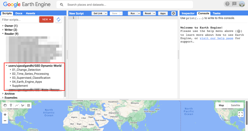
Code Editor After Adding the Workshop Repository
If you do not see the repository in the Reader section, click Refresh repository cache button in your Scripts tab and it will show up.
Module 1: Change Detection
01. Hello World
print('Hello World');

// Variables
var city = 'Bengaluru';
var country = 'India';
print(city, country);

var population = 8400000;
print(population);

// List
var majorCities = ['Mumbai', 'Delhi', 'Chennai', 'Kolkata'];
print(majorCities);

// Dictionary
var cityData = {
  'city': city,
  'population': 8400000,
  'elevation': 930
};
print(cityData);

// Function
var greet = function(name) {
    return 'Hello ' + name;
};
print(greet('World'));

// This is a comment
Exercise
02. Image Collections
/**
 * Function to mask clouds using the Sentinel-2 QA band
 * @param {ee.Image} image Sentinel-2 image
 * @return {ee.Image} cloud masked Sentinel-2 image
 */
function maskS2clouds(image) {
  var qa = image.select('QA60');

  // Bits 10 and 11 are clouds and cirrus, respectively.
  var cloudBitMask = 1 << 10;
  var cirrusBitMask = 1 << 11;

  // Both flags should be set to zero, indicating clear conditions.
  var mask = qa.bitwiseAnd(cloudBitMask).eq(0)
      .and(qa.bitwiseAnd(cirrusBitMask).eq(0));

  return image.updateMask(mask).divide(10000);
}

// Map the function over a month of data and take the median.
// Load Sentinel-2 TOA reflectance data (adjusted for processing changes
// that occurred after 2022-01-25).
var dataset = ee.ImageCollection('COPERNICUS/S2_HARMONIZED')
                  .filterDate('2022-01-01', '2022-01-31')
                  // Pre-filter to get less cloudy granules.
                  .filter(ee.Filter.lt('CLOUDY_PIXEL_PERCENTAGE', 20))
                  .map(maskS2clouds);

var rgbVis = {
  min: 0.0,
  max: 0.3,
  bands: ['B4', 'B3', 'B2'],
};

Map.setCenter(-9.1695, 38.6917, 12);
Map.addLayer(dataset.median(), rgbVis, 'RGB');
Exercise
03. Hello Dynamic World
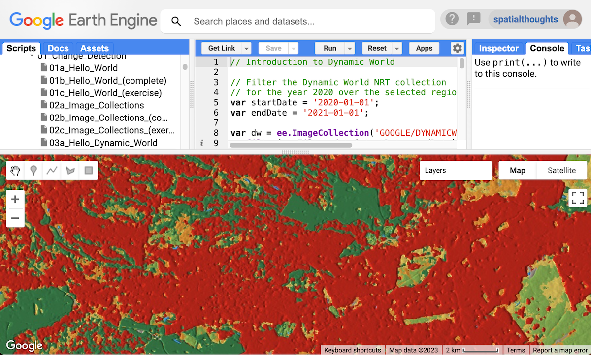
// Introduction to Dynamic World

// Filter the Dynamic World NRT collection
// for the year 2020 over the selected region.
var startDate = '2020-01-01';
var endDate = '2021-01-01';

var dw = ee.ImageCollection('GOOGLE/DYNAMICWORLD/V1')
  .filter(ee.Filter.date(startDate, endDate))

// Create a Mode Composite
var classification = dw.select('label')
var dwComposite = classification.reduce(ee.Reducer.mode());

var dwVisParams = {
  min: 0,
  max: 8,
  palette: ['#419BDF', '#397D49', '#88B053', '#7A87C6',
    '#E49635', '#DFC35A', '#C4281B', '#A59B8F', '#B39FE1']
};

// Clip the composite and add it to the Map
Map.addLayer(dwComposite, dwVisParams, 'Classified Composite')

// Create a Top-1 Probability Hillshade Visualization
var probabilityBands = [
    'water', 'trees', 'grass', 'flooded_vegetation', 'crops',
    'shrub_and_scrub', 'built', 'bare', 'snow_and_ice'
    ];

// Select probability bands
var probabilityCol = dw.select(probabilityBands)

// Create a multi-band image with the average pixel-wise probability
// for each band across the time-period
var meanProbability = probabilityCol.reduce(ee.Reducer.mean())

// Composites have a default projection that is not suitable
// for hillshade computation.
// Set a EPSG:3857 projection with 10m scale
var projection = ee.Projection('EPSG:3857').atScale(10)
var meanProbability = meanProbability.setDefaultProjection(projection)

// Create the Top1 Probability Hillshade
var top1Probability = meanProbability.reduce(ee.Reducer.max())
var top1Confidence = top1Probability.multiply(100).int()
var hillshade = ee.Terrain.hillshade(top1Confidence).divide(255)
var rgbImage = dwComposite.visualize(dwVisParams).divide(255);
var probabilityHillshade = rgbImage.multiply(hillshade)

var hillshadeVisParams = {min:0, max:0.8}
Map.addLayer(probabilityHillshade,
  hillshadeVisParams, 'Probability Hillshade')

Map.setCenter(36.800, -1.266, 12);
Exercise
04. Filtering Image Collections
var geometry = ee.Geometry.Point([36.800, -1.266])
Map.centerObject(geometry, 10)

var s2 = ee.ImageCollection('COPERNICUS/S2_HARMONIZED');

// Filter by metadata
var filtered = s2.filter(ee.Filter.lt('CLOUDY_PIXEL_PERCENTAGE', 35));

// Filter by date
var filtered = s2.filter(ee.Filter.date('2019-01-01', '2020-01-01'));

// Filter by location
var filtered = s2.filter(ee.Filter.bounds(geometry));

// Let's apply all the 3 filters together on the collection

// First apply metadata fileter
var filtered1 = s2.filter(ee.Filter.lt('CLOUDY_PIXEL_PERCENTAGE', 35));
// Apply date filter on the results
var filtered2 = filtered1.filter(
  ee.Filter.date('2019-01-01', '2020-01-01'));
// Lastly apply the location filter
var filtered3 = filtered2.filter(ee.Filter.bounds(geometry));

// Instead of applying filters one after the other, we can 'chain' them
// Use the . notation to apply all the filters together
var filtered = s2.filter(ee.Filter.lt('CLOUDY_PIXEL_PERCENTAGE', 35))
  .filter(ee.Filter.date('2019-01-01', '2020-01-01'))
  .filter(ee.Filter.bounds(geometry));

print(filtered.size());
Exercise
var geometry = ee.Geometry.Point([36.800, -1.266])
Map.centerObject(geometry, 10)

var s2 = ee.ImageCollection('COPERNICUS/S2_HARMONIZED');

var filtered = s2.filter(ee.Filter.lt('CLOUDY_PIXEL_PERCENTAGE', 35))
  .filter(ee.Filter.date('2019-01-01', '2020-01-01'))
  .filter(ee.Filter.bounds(geometry));

print(filtered.size());


// Exercise

// The variable dw has the Dynamic World collection
// Apply the filters to select Dynamic world scenes of interest
// We want to apply the following filters
//    1. Date Filter: ee.Filter.date('2019-01-01', '2020-01-01')
//    2. Bounds Filter ee.Filter.bounds(geometry)
// Apply both the filters and print the number of selected
// Dynamic World scenes

// Tip: Dynamic World is generated for all S2 images with
// CLOUDY_PIXEL_PERCENTAGE < 35. So you don't need to apply
// that filter.
var dw = ee.ImageCollection('GOOGLE/DYNAMICWORLD/V1');
05. Mosaics and Composites
Mean Composite of Built Probability
var geometry = ee.Geometry.Point([36.800, -1.266])
Map.centerObject(geometry, 10)

var s2 = ee.ImageCollection('COPERNICUS/S2_HARMONIZED');

var filtered = s2.filter(ee.Filter.lt('CLOUDY_PIXEL_PERCENTAGE', 30))
  .filter(ee.Filter.date('2019-01-01', '2020-01-01'))
  .filter(ee.Filter.bounds(geometry));

var medianComposite = filtered.median();

var rgbVis = {
  min: 0.0,
  max: 3000,
  bands: ['B4', 'B3', 'B2'],
};

Map.addLayer(medianComposite, rgbVis, 'Median Composite');

var dw = ee.ImageCollection('GOOGLE/DYNAMICWORLD/V1');

var dwFiltered = dw
    .filter(ee.Filter.date('2019-01-01', '2020-01-01'))
    .filter(ee.Filter.bounds(geometry));

var probabilityBands = [
  'water', 'trees', 'grass', 'flooded_vegetation', 'crops', 'shrub_and_scrub',
  'built', 'bare', 'snow_and_ice'
];

var dwProbability = dwFiltered.select(probabilityBands);

var dwComposite = dwProbability.mean();

var dwVis = {
  min: 0,
  max: 1,
  bands: ['built'],
  palette: ['white', 'red']
};

Map.addLayer(dwComposite, dwVis, 'Built Probability')
Exercise
06. Feature Collections
var admin2 = ee.FeatureCollection('FAO/GAUL_SIMPLIFIED_500m/2015/level2');
var filtered = admin2.filter(ee.Filter.eq('ADM0_NAME', 'Kenya'));

var visParams = {'color': 'red'};
Map.addLayer(filtered, visParams, 'Selected Counties');
Exercise
07. Import
// Let's import some data to Earth Engine

// We will upload the 'Kenya Admin Level 4 Boundaries'
// https://data.humdata.org/dataset/kenya-admin-level-4-boundaries

// Download the shapefile from https://bit.ly/kenya-admin4-shp
// Unzip and upload

// Import the collection
var admin4 = ee.FeatureCollection('users/ujavalgandhi/kenya/kenya_admin4');

// Visualize the collection
Map.addLayer(admin4, {color: 'blue'}, 'Admin4');
Exercise
// Import the collection
var admin4 = ee.FeatureCollection('users/ujavalgandhi/kenya/kenya_admin4');

// Visualize the collection
Map.addLayer(admin4, {color: 'blue'}, 'Admin4');

// Apply a filter to select an admin4 region of your choice
// Hint: The admin4 names are in the property 'LOCANAME'

// Add the selected county to the Map in 'red' color
08. Clipping
var s2 = ee.ImageCollection("COPERNICUS/S2_HARMONIZED");
var admin4 = ee.FeatureCollection('users/ujavalgandhi/kenya/kenya_admin4');
var filtered = admin4.filter(ee.Filter.eq('LOCNAME', 'LANGATA'));
var geometry = filtered.geometry();
Map.centerObject(geometry);

var rgbVis = {
  min: 0.0,
  max: 3000,
  bands: ['B4', 'B3', 'B2'],
};
var filtered = s2.filter(ee.Filter.lt('CLOUDY_PIXEL_PERCENTAGE', 30))
  .filter(ee.Filter.date('2019-01-01', '2020-01-01'))
  .filter(ee.Filter.bounds(geometry));

var image = filtered.median();


var clipped = image.clip(geometry);
Map.addLayer(clipped, rgbVis, 'Clipped Composite');
Exercise
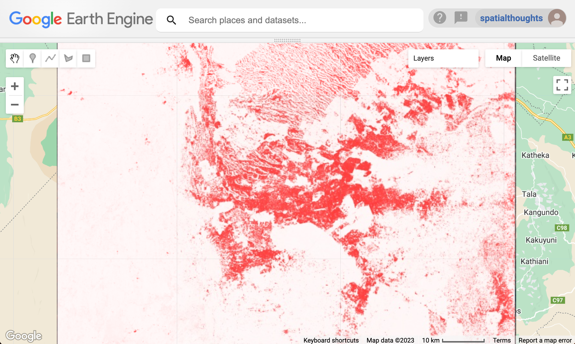
09. Change Detection
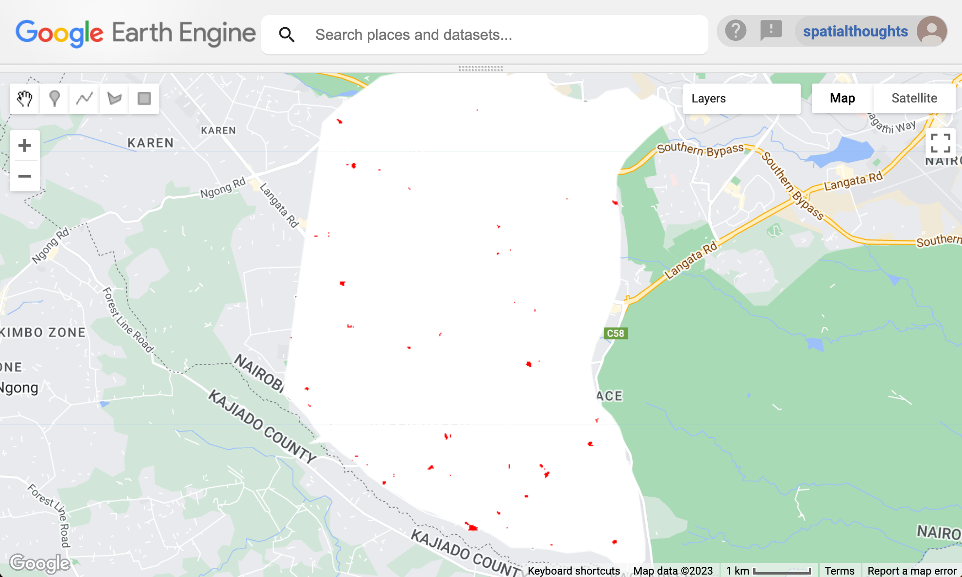
Newly Urbanized Areas Detected in Langata, Nairobi
var s2 = ee.ImageCollection("COPERNICUS/S2_HARMONIZED");
var admin4 = ee.FeatureCollection('users/ujavalgandhi/kenya/kenya_admin4');
var filtered = admin4.filter(ee.Filter.eq('LOCNAME', 'LANGATA'));
var geometry = filtered.geometry();
Map.centerObject(geometry);

// Detect newly urbanized regions from the year 2019 to 2020.
var beforeYear = 2020;
var afterYear = 2022;

// Create start and end dates for the before and after periods.
var beforeStart = ee.Date.fromYMD(beforeYear, 1 , 1);
var beforeEnd = beforeStart.advance(1, 'year');

var afterStart = ee.Date.fromYMD(afterYear, 1 , 1);
var afterEnd = afterStart.advance(1, 'year');


var rgbVis = {
  min: 0.0,
  max: 3000,
  bands: ['B4', 'B3', 'B2'],
};

// Create a median composite from sentinel-2 images.
var beforeS2 = s2
.filter(ee.Filter.lt('CLOUDY_PIXEL_PERCENTAGE', 35))
.filter(ee.Filter.date(beforeStart, beforeEnd))
.median();

var afterS2 = s2
  .filter(ee.Filter.lt('CLOUDY_PIXEL_PERCENTAGE', 35))
  .filter(ee.Filter.date(afterStart, afterEnd))
  .median();

var s2VisParams = {bands: ['B4', 'B3', 'B2'], min: 0, max: 3000};
Map.addLayer(beforeS2.clip(geometry), s2VisParams, 'Before S2');
Map.addLayer(afterS2.clip(geometry), s2VisParams, 'After S2');


// Filter the Dynamic World collection and select the 'built' band.
var dw = ee.ImageCollection('GOOGLE/DYNAMICWORLD/V1')
  .filterBounds(geometry).select('built');

// Create a mean composite indicating the average probability through the year.
var beforeDw = dw
  .filter(ee.Filter.date(beforeStart, beforeEnd))
  .mean();

var afterDw = dw
  .filter(ee.Filter.date(afterStart, afterEnd))
  .mean();

// Select all pixels that are
// < 0.2 'built' probability before
// > 0.5 'built' probability after


// Filter the Dynamic World collection and select the 'built' band.
var dw = ee.ImageCollection('GOOGLE/DYNAMICWORLD/V1')
  .filterBounds(geometry).select('built');

// Create a mean composite indicating the average probability through the year.
var beforeDw = dw.filterDate(beforeStart, beforeEnd).mean();

var afterDw = dw.filterDate(afterStart, afterEnd).mean();

// Select all pixels that are
// < 0.2 'built' probability before
// > 0.5 'built' probability after
var newUrban = beforeDw.lt(0.2).and(afterDw.gt(0.5));

var changeVisParams = {min: 0, max: 1, palette: ['white', 'red']};
Map.addLayer(newUrban.clip(geometry), changeVisParams, 'New Urban');
Exercise
10. Convert to Vector
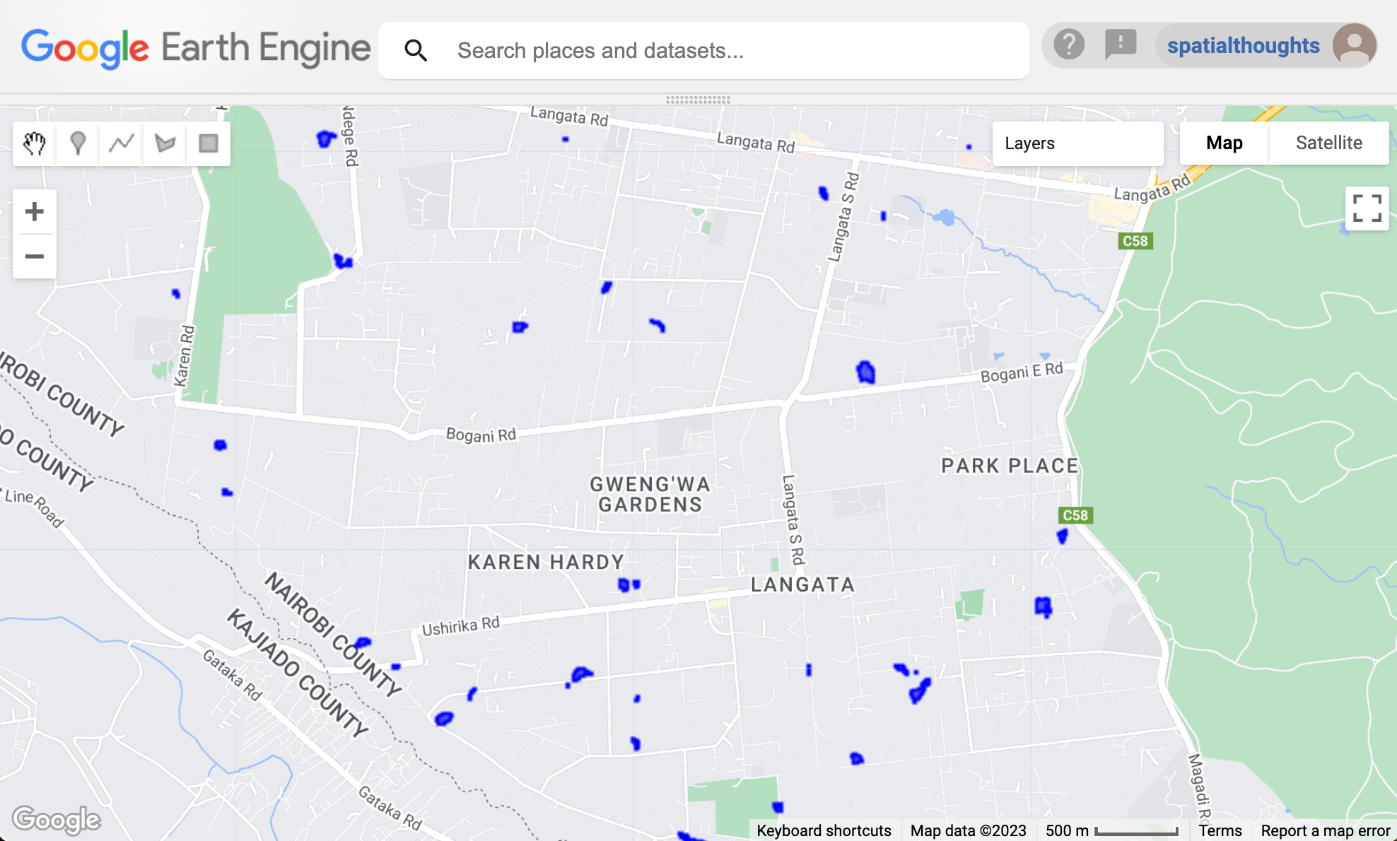
Vectorized Polygons for Newly Urbanized Areas
var s2 = ee.ImageCollection("COPERNICUS/S2_HARMONIZED");
var admin4 = ee.FeatureCollection('users/ujavalgandhi/kenya/kenya_admin4');
var filtered = admin4.filter(ee.Filter.eq('LOCNAME', 'LANGATA'));
var geometry = filtered.geometry();
Map.centerObject(geometry);

// Detect newly urbanized regions from the year 2019 to 2020.
var beforeYear = 2020;
var afterYear = 2022;

// Create start and end dates for the before and after periods.
var beforeStart = ee.Date.fromYMD(beforeYear, 1 , 1);
var beforeEnd = beforeStart.advance(1, 'year');

var afterStart = ee.Date.fromYMD(afterYear, 1 , 1);
var afterEnd = afterStart.advance(1, 'year');


var rgbVis = {
  min: 0.0,
  max: 3000,
  bands: ['B4', 'B3', 'B2'],
};

// Create a median composite from sentinel-2 images.
var beforeS2 = s2
.filter(ee.Filter.lt('CLOUDY_PIXEL_PERCENTAGE', 35))
.filter(ee.Filter.date(beforeStart, beforeEnd))
.median();

var afterS2 = s2
  .filter(ee.Filter.lt('CLOUDY_PIXEL_PERCENTAGE', 35))
  .filter(ee.Filter.date(afterStart, afterEnd))
  .median();

var s2VisParams = {bands: ['B4', 'B3', 'B2'], min: 0, max: 3000};
Map.addLayer(beforeS2.clip(geometry), s2VisParams, 'Before S2');
Map.addLayer(afterS2.clip(geometry), s2VisParams, 'After S2');


// Filter the Dynamic World collection and select the 'built' band.
var dw = ee.ImageCollection('GOOGLE/DYNAMICWORLD/V1')
  .filterBounds(geometry).select('built');

// Create a mean composite indicating the average probability through the year.
var beforeDw = dw
  .filter(ee.Filter.date(beforeStart, beforeEnd))
  .mean();

var afterDw = dw
  .filter(ee.Filter.date(afterStart, afterEnd))
  .mean();

// Select all pixels that are
// < 0.2 'built' probability before
// > 0.5 'built' probability after


// Filter the Dynamic World collection and select the 'built' band.
var dw = ee.ImageCollection('GOOGLE/DYNAMICWORLD/V1')
  .filterBounds(geometry).select('built');

// Create a mean composite indicating the average probability through the year.
var beforeDw = dw.filterDate(beforeStart, beforeEnd).mean();

var afterDw = dw.filterDate(afterStart, afterEnd).mean();

// Select all pixels that are
// < 0.2 'built' probability before
// > 0.5 'built' probability after
var newUrban = beforeDw.lt(0.2).and(afterDw.gt(0.5));

var changeVisParams = {min: 0, max: 1, palette: ['white', 'red']};
Map.addLayer(newUrban.clip(geometry), changeVisParams, 'New Urban');

// Convert the raster image to vector
// We use .selfMask() function to remove all pixels with 0 values
var newUrbanMasked = newUrban.selfMask();

// Convert to polygons
var newUrbanVector = newUrbanMasked.reduceToVectors({
  geometry: geometry,
  scale: 10,
  eightConnected: false,
  maxPixels: 1e10,
  tileScale: 16
});
Map.addLayer(newUrbanVector, {color:'blue'}, 'New Urban Polygons');
Exercise
11. Export
var s2 = ee.ImageCollection("COPERNICUS/S2_HARMONIZED");
var admin4 = ee.FeatureCollection('users/ujavalgandhi/kenya/kenya_admin4');
var filtered = admin4.filter(ee.Filter.eq('LOCNAME', 'LANGATA'));
var geometry = filtered.geometry();
Map.centerObject(geometry);

// Detect newly urbanized regions from the year 2019 to 2020.
var beforeYear = 2020;
var afterYear = 2022;

// Create start and end dates for the before and after periods.
var beforeStart = ee.Date.fromYMD(beforeYear, 1 , 1);
var beforeEnd = beforeStart.advance(1, 'year');

var afterStart = ee.Date.fromYMD(afterYear, 1 , 1);
var afterEnd = afterStart.advance(1, 'year');


var rgbVis = {
  min: 0.0,
  max: 3000,
  bands: ['B4', 'B3', 'B2'],
};

// Create a median composite from sentinel-2 images.
var beforeS2 = s2
.filter(ee.Filter.lt('CLOUDY_PIXEL_PERCENTAGE', 35))
.filter(ee.Filter.date(beforeStart, beforeEnd))
.median();

var afterS2 = s2
  .filter(ee.Filter.lt('CLOUDY_PIXEL_PERCENTAGE', 35))
  .filter(ee.Filter.date(afterStart, afterEnd))
  .median();

var s2VisParams = {bands: ['B4', 'B3', 'B2'], min: 0, max: 3000};
Map.addLayer(beforeS2.clip(geometry), s2VisParams, 'Before S2');
Map.addLayer(afterS2.clip(geometry), s2VisParams, 'After S2');


// Filter the Dynamic World collection and select the 'built' band.
var dw = ee.ImageCollection('GOOGLE/DYNAMICWORLD/V1')
  .filterBounds(geometry).select('built');

// Create a mean composite indicating the average probability through the year.
var beforeDw = dw
  .filter(ee.Filter.date(beforeStart, beforeEnd))
  .mean();

var afterDw = dw
  .filter(ee.Filter.date(afterStart, afterEnd))
  .mean();

// Select all pixels that are
// < 0.2 'built' probability before
// > 0.5 'built' probability after


// Filter the Dynamic World collection and select the 'built' band.
var dw = ee.ImageCollection('GOOGLE/DYNAMICWORLD/V1')
  .filterBounds(geometry).select('built');

// Create a mean composite indicating the average probability through the year.
var beforeDw = dw.filterDate(beforeStart, beforeEnd).mean();

var afterDw = dw.filterDate(afterStart, afterEnd).mean();

// Select all pixels that are
// < 0.2 'built' probability before
// > 0.5 'built' probability after
var newUrban = beforeDw.lt(0.2).and(afterDw.gt(0.5)).rename('change');

var changeVisParams = {min: 0, max: 1, palette: ['white', 'red']};
Map.addLayer(newUrban.clip(geometry), changeVisParams, 'New Urban');

// Convert the raster image to vector
// We use .selfMask() function to remove all pixels with 0 values
var newUrbanMasked = newUrban.selfMask();

// Convert to polygons
var newUrbanVector = newUrbanMasked.reduceToVectors({
  geometry: geometry,
  scale: 10,
  eightConnected: false,
  maxPixels: 1e10,
  tileScale: 16
});
Map.addLayer(newUrbanVector, {color:'blue'}, 'New Urban Polygons');

// Select bands for export
var beforeS2Export = beforeS2.select('B.*').clip(geometry);
var afterS2Export = afterS2.select('B.*').clip(geometry);

// Option 1: Export Raw Images
// Suitable for further analysis
Export.image.toDrive({
    image: beforeS2Export,
    description: 'Before_Composite',
    folder: 'earthengine',
    fileNamePrefix: 'before_composite',
    region: geometry,
    scale: 10,
    maxPixels: 1e9
});

Export.image.toDrive({
    image: afterS2Export,
    description: 'After_Composite',
    folder: 'earthengine',
    fileNamePrefix: 'after_composite',
    region: geometry,
    scale: 10,
    maxPixels: 1e9
});

// Option 2: Export Visualized Images
// Suitable for viewing and embedding

var beforeS2ExportVisualized = beforeS2Export.visualize(rgbVis);
var afterS2ExportVisualized = afterS2Export.visualize(rgbVis);

Export.image.toDrive({
    image: beforeS2ExportVisualized,
    description: 'Before_Composite_Visualized',
    folder: 'earthengine',
    fileNamePrefix: 'before_composite_visualized',
    region: geometry,
    scale: 10,
    maxPixels: 1e9
});

Export.image.toDrive({
    image: afterS2ExportVisualized,
    description: 'After_Composite_Visualized',
    folder: 'earthengine',
    fileNamePrefix: 'after_composite_visualized',
    region: geometry,
    scale: 10,
    maxPixels: 1e9
});

// Export the Polygons
Export.table.toDrive({
  collection: newUrbanVector,
  description: 'New_Urban_Polygons',
  folder: 'earthengine',
  fileNamePrefix: 'new_urban_polygons',
  fileFormat: 'SHP'
})
Exercise
Quiz - Module 1
This is a short quiz to test your understanding of the Module 1 concepts.
Module 2: Supervised Classification

01. Basic Supervised Classification
var s2 = ee.ImageCollection('COPERNICUS/S2_SR_HARMONIZED');

// The following collections were created using the
// Drawing Tools in the code editor and exported as assets.
var mangroves = ee.FeatureCollection('users/ujavalgandhi/kenya/basic_gcps_mangroves');
var water = ee.FeatureCollection('users/ujavalgandhi/kenya/basic_gcps_water');
var other = ee.FeatureCollection('users/ujavalgandhi/kenya/basic_gcps_other');

var geometry = ee.Geometry.Polygon([[
  [39.4926285922204, -4.398315001988073],
  [39.4926285922204, -4.4739620180298845],
  [39.54910518523798, -4.4739620180298845],
  [39.54910518523798, -4.398315001988073]
]]);

var filtered = s2
  .filter(ee.Filter.lt('CLOUDY_PIXEL_PERCENTAGE', 35))
  .filter(ee.Filter.date('2020-01-01', '2021-01-01'))
  .filter(ee.Filter.bounds(geometry))
  .select('B.*');

var composite = filtered.median();

// Display the input composite.
var rgbVis = {min: 0.0, max: 3000, bands: ['B4', 'B3', 'B2']};
var swirVis = {min: 300, max: 4000, bands: ['B11', 'B8', 'B4']};
Map.centerObject(geometry);
Map.addLayer(composite.clip(geometry), rgbVis, 'S2 Composite (RGB)');
Map.addLayer(composite.clip(geometry), swirVis, 'S2 Composite (False Color)');

var gcps = mangroves.merge(water).merge(other);

// Overlay the point on the image to get training data.
var training = composite.sampleRegions({
  collection: gcps,
  properties: ['landcover'],
  scale: 10
});


// Train a classifier.
var classifier = ee.Classifier.smileRandomForest(50).train({
  features: training,
  classProperty: 'landcover',
  inputProperties: composite.bandNames()
});
// // Classify the image.
var classified = composite.classify(classifier);
// Choose a 3-color palette
// Assign a color for each class in the following order
// Mangrove, Water, Other
var palette = ['green', 'blue', 'gray'];

Map.addLayer(classified.clip(geometry), {min: 1, max: 3, palette: palette}, '2020');
Exercise
02. Supervised Classification with Dynamic World Bands
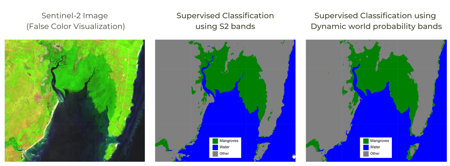
Comparison of classification results using S2 vs DW bands
// Create a Sentinel-2 Compsite for Visualization
var s2 = ee.ImageCollection('COPERNICUS/S2_SR_HARMONIZED');

// The following collections were created using the
// Drawing Tools in the code editor and exported as assets.
var mangroves = ee.FeatureCollection('users/ujavalgandhi/kenya/basic_gcps_mangroves');
var water = ee.FeatureCollection('users/ujavalgandhi/kenya/basic_gcps_water');
var other = ee.FeatureCollection('users/ujavalgandhi/kenya/basic_gcps_other');

var geometry = ee.Geometry.Polygon([[
  [39.4926285922204, -4.398315001988073],
  [39.4926285922204, -4.4739620180298845],
  [39.54910518523798, -4.4739620180298845],
  [39.54910518523798, -4.398315001988073]
]]);

var filtered = s2
  .filter(ee.Filter.lt('CLOUDY_PIXEL_PERCENTAGE', 35))
  .filter(ee.Filter.date('2020-01-01', '2021-01-01'))
  .filter(ee.Filter.bounds(geometry))
  .select('B.*');

var composite = filtered.median();
print(composite)
// Display the input composite.
var rgbVis = {min: 0.0, max: 3000, bands: ['B4', 'B3', 'B2']};
Map.centerObject(geometry);
Map.addLayer(composite.clip(geometry), rgbVis, 'S2 Composite (RGB)');

var gcps = mangroves.merge(water).merge(other);

// ####### S2-based Supervised Classification #######

// Overlay the point on the image to get training data.
var training = composite.sampleRegions({
  collection: gcps,
  properties: ['landcover'],
  scale: 10
});


// Train a classifier.
var classifier = ee.Classifier.smileRandomForest(50).train({
  features: training,
  classProperty: 'landcover',
  inputProperties: composite.bandNames()
});
// // Classify the image.
var classified = composite.classify(classifier);
// Choose a 3-color palette
// Assign a color for each class in the following order
// Mangrove, Water, Other
var palette = ['green', 'blue', 'gray'];

Map.addLayer(classified.clip(geometry), {min: 1, max: 3, palette: palette}, 'S2 Classification');

// ####### DW-based Supervised Classification #######

// Create a Dynamic World Composite to use as input to classification
var probabilityBands = [
    'water', 'trees', 'grass', 'flooded_vegetation', 'crops',
    'shrub_and_scrub', 'built', 'bare', 'snow_and_ice'
    ];

var dw = ee.ImageCollection('GOOGLE/DYNAMICWORLD/V1')

var dwfiltered = dw
  .filter(ee.Filter.date('2020-01-01', '2021-01-01'))
  .filter(ee.Filter.bounds(geometry))
  .select(probabilityBands)

var dwComposite = dwfiltered.mean();

// Overlay the point on the image to get training data.
var training = dwComposite.sampleRegions({
  collection: gcps,
  properties: ['landcover'],
  scale: 10
});


// Train a classifier.
var classifier = ee.Classifier.smileRandomForest(50).train({
  features: training,
  classProperty: 'landcover',
  inputProperties: dwComposite.bandNames()
});
// // Classify the Dynamic World image.
var classified = dwComposite.classify(classifier);
// Choose a 3-color palette
// Assign a color for each class in the following order
// Mangrove, Water, Other
var palette = ['green', 'blue', 'gray'];

Map.addLayer(
  classified.clip(geometry),
  {min: 1, max: 3, palette: palette},
  'DW Classified');
Exercise
03. Accuracy Assessment
// We now switch to another example that has a lot more training samples
// and tries to classify the entire coastline of Kenya into
// mangroves, water and other classes.
// See the Supplement folder in the repository to see the script
// that was used to generate this training data.
var gcps = ee.FeatureCollection('users/ujavalgandhi/kenya/mangroves_gcps');
var coastline = ee.FeatureCollection('users/ujavalgandhi/kenya/kenya_coastline');

var geometry = coastline.geometry();
Map.centerObject(geometry, 10);
Map.addLayer(coastline.draw({color: '#fff7bc', strokeWidth: 1}), {}, 'Area of Interest');

var mangroves = gcps.filter(ee.Filter.eq('landcover', 1));
var water = gcps.filter(ee.Filter.eq('landcover', 2));
var other = gcps.filter(ee.Filter.eq('landcover', 3));
Map.addLayer(mangroves, {color: 'green'}, 'Magrove GCPs', false);
Map.addLayer(water, {color: 'blue'}, 'Water GCPs', false);
Map.addLayer(other, {color: 'gray'}, 'Other GCPs', false);

// Create Sentinel-2 Composite
var s2 = ee.ImageCollection('COPERNICUS/S2_SR_HARMONIZED');

var filtered = s2
.filter(ee.Filter.lt('CLOUDY_PIXEL_PERCENTAGE', 35))
  .filter(ee.Filter.date('2020-01-01', '2021-01-01'))
  .filter(ee.Filter.bounds(geometry))
  .select('B.*');

var composite = filtered.median();

// Display the input composite.
var rgbVis = {min: 0, max: 0.3, bands: ['B4', 'B3', 'B2']};
var swirVis = {min: 0.03, max: 0.4, bands: ['B11', 'B8', 'B4']};
Map.centerObject(geometry);
Map.addLayer(composite.clip(geometry), rgbVis, 'S2 Composite (RGB)', false);
Map.addLayer(composite.clip(geometry), swirVis, 'S2 Composite (False Color)');

//**************************************************************************
// Accuracy Assessment
//**************************************************************************

// Add a random column and split the GCPs into training and validation set
var gcps = gcps.randomColumn();

var trainingGcp = gcps.filter(ee.Filter.lt('random', 0.6));
var validationGcp = gcps.filter(ee.Filter.gte('random', 0.6));

print('Total GCPs', gcps.size());
print('Training GCPs', trainingGcp.size());
print('Validation GCPs', validationGcp.size());

var training = composite.sampleRegions({
    collection: trainingGcp,
    properties: ['landcover'],
    scale: 10,
    tileScale: 16
});

print('Training Feature', training.first());

// Train a classifier.
var classifier = ee.Classifier.smileRandomForest(50)
  .train({
    features: training,
    classProperty: 'landcover',
    inputProperties: composite.bandNames()
  });

// Classify the image.
var classified = composite.classify(classifier);

// Use classification map to assess accuracy using the validation fraction
// of the overall training set created above.
var test = classified.sampleRegions({
  collection: validationGcp,
  properties: ['landcover'],
  tileScale: 16,
  scale: 10,
});

var testConfusionMatrix = test.errorMatrix('landcover', 'classification');
print('Confusion Matrix', testConfusionMatrix);
print('Test Accuracy', testConfusionMatrix.accuracy());

var classVis = {min:1, max:3, palette: ['green', 'blue', 'gray']}
Map.addLayer(classified.clip(geometry), classVis, '2020 (S2)');
Exercise
04. Improving the Classification
var gcps = ee.FeatureCollection('users/ujavalgandhi/kenya/mangroves_gcps');
var coastline = ee.FeatureCollection('users/ujavalgandhi/kenya/kenya_coastline');

var geometry = coastline.geometry();
Map.centerObject(geometry, 10);
Map.addLayer(coastline.draw({color: '#fff7bc', strokeWidth: 1}), {}, 'Area of Interest');

var mangroves = gcps.filter(ee.Filter.eq('landcover', 1));
var water = gcps.filter(ee.Filter.eq('landcover', 2));
var other = gcps.filter(ee.Filter.eq('landcover', 3));
Map.addLayer(mangroves, {color: 'green'}, 'Magrove GCPs', false);
Map.addLayer(water, {color: 'blue'}, 'Water GCPs', false);
Map.addLayer(other, {color: 'gray'}, 'Other GCPs', false);

// Create Sentinel-2 Composite
var s2 = ee.ImageCollection('COPERNICUS/S2_SR_HARMONIZED');

// Function to remove cloud and snow pixels from Sentinel-2 SR image
function maskS2clouds(image) {
  var qa = image.select('QA60');
  var cloudBitMask = 1 << 10;
  var cirrusBitMask = 1 << 11;
  var mask = qa.bitwiseAnd(cloudBitMask).eq(0).and(
            qa.bitwiseAnd(cirrusBitMask).eq(0));
  return image.updateMask(mask)
      .select('B.*')
      .multiply(0.0001)
      .copyProperties(image, ['system:time_start']);
}

var filtered = s2
.filter(ee.Filter.lt('CLOUDY_PIXEL_PERCENTAGE', 35))
  .filter(ee.Filter.date('2020-01-01', '2021-01-01'))
  .filter(ee.Filter.bounds(geometry))
  .map(maskS2clouds)
  .select('B.*');

var composite = filtered.median();

// Display the input composite.
var rgbVis = {min: 0, max: 0.3, bands: ['B4', 'B3', 'B2']};
var swirVis = {min: 0.03, max: 0.4, bands: ['B11', 'B8', 'B4']};
Map.centerObject(geometry);
Map.addLayer(composite.clip(geometry), rgbVis, 'S2 Composite (RGB)', false);
Map.addLayer(composite.clip(geometry), swirVis, 'S2 Composite (False Color)');


// Create Dynamic World Probability Bands Composite

// Dynamic World

// Create a Probability Hillshade Visualization
var probabilityBands = [
    'water', 'trees', 'grass', 'flooded_vegetation', 'crops',
    'shrub_and_scrub', 'built', 'bare', 'snow_and_ice'
    ];

var dw = ee.ImageCollection('GOOGLE/DYNAMICWORLD/V1')

var dwfiltered = dw
  .filter(ee.Filter.date('2020-01-01', '2021-01-01'))
  .filter(ee.Filter.bounds(geometry))
  .select(probabilityBands)

var probabilityImage = dwfiltered.mean();

//**************************************************************************
// Accuracy Assessment
//**************************************************************************

// Add a random column and split the GCPs into training and validation set
var gcps = gcps.randomColumn();

var trainingGcp = gcps.filter(ee.Filter.lt('random', 0.6));
var validationGcp = gcps.filter(ee.Filter.gte('random', 0.6));

print('Total GCPs', gcps.size());
print('Training GCPs', trainingGcp.size());
print('Validation GCPs', validationGcp.size());

// Function to train a classifier and classify an input image
var classifyImage = function(image, label) {

  // Overlay the point on the image to get training data.
  var training = image.sampleRegions({
    collection: trainingGcp,
    properties: ['landcover'],
    scale: 10,
    tileScale: 16
  });
  print(label + ' Training Feature', training.first())
  // Train a classifier.
  var classifier = ee.Classifier.smileRandomForest(50)
  .train({
    features: training,
    classProperty: 'landcover',
    inputProperties: image.bandNames()
  });

  // Classify the image.
  var classified = image.classify(classifier);


  // Use classification map to assess accuracy using the validation fraction
  // of the overall training set created above.
  var test = classified.sampleRegions({
    collection: validationGcp,
    properties: ['landcover'],
    tileScale: 16,
    scale: 10,
  });

  var testConfusionMatrix = test.errorMatrix('landcover', 'classification')
  print(label + ' Confusion Matrix', testConfusionMatrix);
  print(label + ' Test Accuracy', testConfusionMatrix.accuracy());

  return classified;

}

// Classify S2 Composite
var classified = classifyImage(composite, 'S2 Bands');
var classVis = {min:1, max:3, palette: ['green', 'blue', 'gray']}

Map.addLayer(classified.clip(geometry), classVis, '2020 (S2)');

// Classify DW Composite
var classified = classifyImage(probabilityImage, 'DW Bands');
Map.addLayer(classified.clip(geometry), classVis, '2020 (DW)');
Exercise
05. Exporting Classification Results
var gcps = ee.FeatureCollection('users/ujavalgandhi/kenya/mangroves_gcps');
var coastline = ee.FeatureCollection('users/ujavalgandhi/kenya/kenya_coastline');

var geometry = coastline.geometry();
Map.centerObject(geometry, 10);
Map.addLayer(coastline.draw({color: '#fff7bc', strokeWidth: 1}), {}, 'Area of Interest');

var mangroves = gcps.filter(ee.Filter.eq('landcover', 1));
var water = gcps.filter(ee.Filter.eq('landcover', 2));
var other = gcps.filter(ee.Filter.eq('landcover', 3));
Map.addLayer(mangroves, {color: 'green'}, 'Magrove GCPs', false);
Map.addLayer(water, {color: 'blue'}, 'Water GCPs', false);
Map.addLayer(other, {color: 'gray'}, 'Other GCPs', false);

// Create Sentinel-2 Composite
var s2 = ee.ImageCollection('COPERNICUS/S2_SR_HARMONIZED');

// Function to remove cloud and snow pixels from Sentinel-2 SR image
function maskS2clouds(image) {
  var qa = image.select('QA60');
  var cloudBitMask = 1 << 10;
  var cirrusBitMask = 1 << 11;
  var mask = qa.bitwiseAnd(cloudBitMask).eq(0).and(
            qa.bitwiseAnd(cirrusBitMask).eq(0));
  return image.updateMask(mask)
      .select('B.*')
      .multiply(0.0001)
      .copyProperties(image, ['system:time_start']);
}

var filtered = s2
.filter(ee.Filter.lt('CLOUDY_PIXEL_PERCENTAGE', 35))
  .filter(ee.Filter.date('2020-01-01', '2021-01-01'))
  .filter(ee.Filter.bounds(geometry))
  .map(maskS2clouds)
  .select('B.*');

var composite = filtered.median();

// Display the input composite.
var rgbVis = {min: 0, max: 0.3, bands: ['B4', 'B3', 'B2']};
var swirVis = {min: 0.03, max: 0.4, bands: ['B11', 'B8', 'B4']};
Map.centerObject(geometry);
Map.addLayer(composite.clip(geometry), rgbVis, 'S2 Composite (RGB)', false);
Map.addLayer(composite.clip(geometry), swirVis, 'S2 Composite (False Color)');


// Create Dynamic World Probability Bands Composite

// Dynamic World

// Create a Probability Hillshade Visualization
var probabilityBands = [
    'water', 'trees', 'grass', 'flooded_vegetation', 'crops',
    'shrub_and_scrub', 'built', 'bare', 'snow_and_ice'
    ];

var dw = ee.ImageCollection('GOOGLE/DYNAMICWORLD/V1')

var dwfiltered = dw
  .filter(ee.Filter.date('2020-01-01', '2021-01-01'))
  .filter(ee.Filter.bounds(geometry))
  .select(probabilityBands)

var probabilityImage = dwfiltered.mean();

//**************************************************************************
// Accuracy Assessment
//**************************************************************************

// Add a random column and split the GCPs into training and validation set
var gcps = gcps.randomColumn();

var trainingGcp = gcps.filter(ee.Filter.lt('random', 0.6));
var validationGcp = gcps.filter(ee.Filter.gte('random', 0.6));

print('Total GCPs', gcps.size());
print('Training GCPs', trainingGcp.size());
print('Validation GCPs', validationGcp.size());

// Function to train a classifier and classify an input image
var classifyImage = function(image, label) {

  // Overlay the point on the image to get training data.
  var training = image.sampleRegions({
    collection: trainingGcp,
    properties: ['landcover'],
    scale: 10,
    tileScale: 16
  });
  print(label + ' Training Feature', training.first())
  // Train a classifier.
  var classifier = ee.Classifier.smileRandomForest(50)
  .train({
    features: training,
    classProperty: 'landcover',
    inputProperties: image.bandNames()
  });

  // Classify the image.
  var classified = image.classify(classifier);


  // Use classification map to assess accuracy using the validation fraction
  // of the overall training set created above.
  var test = classified.sampleRegions({
    collection: validationGcp,
    properties: ['landcover'],
    tileScale: 16,
    scale: 10,
  });

  var testConfusionMatrix = test.errorMatrix('landcover', 'classification')
  print(label + ' Confusion Matrix', testConfusionMatrix);
  print(label + ' Test Accuracy', testConfusionMatrix.accuracy());

  //**************************************************************************
  // Exporting Results
  //**************************************************************************

  // Create a Feature with null geometry and the value we want to export.
  // Use .array() to convert Confusion Matrix to an Array so it can be
  // exported in a CSV file
  var fc = ee.FeatureCollection([
    ee.Feature(null, {
      'accuracy': testConfusionMatrix.accuracy(),
      'matrix': testConfusionMatrix.array()
    })
  ]);

  print(label + ' Export Collection', fc);

  Export.table.toDrive({
    collection: fc,
    description: label + '_Accuracy_Export',
    folder: 'earthengine',
    fileNamePrefix: label + '_accuracy',
    fileFormat: 'CSV'
  });

  // Use the Export.image.toAsset() function to export the
  // classified image as a Earth Engine Asset.

  // For images with discrete pixel values, we must set the
  // pyramidingPolicy to 'mode'.
  Export.image.toAsset({
    image: classified.clip(geometry),
    description: label + '_Asset_Export',
    assetId: label + '_classified',
    pyramidingPolicy:{'.default': 'mode'},
    region: geometry,
    scale: 10,
    maxPixels: 1e10
  });

  return classified;

}

// Classify S2 Composite
var classified = classifyImage(composite, 'S2_Bands');
var classVis = {min:1, max:3, palette: ['green', 'blue', 'gray']}

Map.addLayer(classified.clip(geometry), classVis, '2020 (S2)');

// Classify DW Composite
var classified = classifyImage(probabilityImage, 'DW_Bands');
Map.addLayer(classified.clip(geometry), classVis, '2020 (DW)');
Exercise
06. Calculating Area
/**** Start of imports. If edited, may not auto-convert in the playground. ****/
var geometry =
    /* color: #98ff00 */
    /* shown: false */
    /* displayProperties: [
      {
        "type": "rectangle"
      }
    ] */
    ee.Geometry.Polygon(
        [[[39.4926285922204, -4.398315001988073],
          [39.4926285922204, -4.4739620180298845],
          [39.54910518523798, -4.4739620180298845],
          [39.54910518523798, -4.398315001988073]]], null, false),
    classified = ee.Image("users/ujavalgandhi/kenya/mangroves_classified");
/***** End of imports. If edited, may not auto-convert in the playground. *****/
Map.addLayer(geometry, {color: 'blue'}, 'AOI');

var palette = ['green', 'blue', 'gray'];
Map.addLayer(classified, {min: 1, max: 3, palette: palette}, 'Classified Image');

// Calculate Area for Vectors

// .area() function calculates the area in square meters
var aoiArea = geometry.area({maxError: 1});

// We can cast the result to a ee.Number() and calculate the
// area in square kilometers
var aoiAreaSqKm = ee.Number(aoiArea).divide(1e6).round();
print(aoiAreaSqKm);

// Area Calculation for Images
var mangroves = classified.eq(1);
// If the image contains values 0 or 1, we can calculate the
// total area using reduceRegion() function

// The result of .eq() operation is a binary image with pixels
// values of 1 where the condition matched and 0 where it didn't
Map.addLayer(mangroves, {min:0, max:1, palette: ['white', 'black']}, 'Mangroves');

// Since our image has only 0 and 1 pixel values, the vegetation
// pixels will have values equal to their area
var areaImage = mangroves.multiply(ee.Image.pixelArea());


// Now that each pixel for vegetation class in the image has the value
// equal to its area, we can sum up all the values in the region
// to get the total green cover.

var area = areaImage.reduceRegion({
  reducer: ee.Reducer.sum(),
  geometry: geometry,
  scale: 10,
  maxPixels: 1e10
});
// The result of the reduceRegion() function is a dictionary with the key
// being the band name. We can extract the area number and convert it to
// square kilometers
var mangrovesAreaSqKm = area.getNumber('classification').divide(1e6).round();
print(mangrovesAreaSqKm);
Exercise
var geometry = ee.Geometry.Polygon([[
  [39.4926285922204, -4.398315001988073],
  [39.4926285922204, -4.4739620180298845],
  [39.54910518523798, -4.4739620180298845],
  [39.54910518523798, -4.398315001988073]
]]);
var classified = ee.Image('users/ujavalgandhi/kenya/mangroves_classified');

Map.addLayer(geometry, {color: 'blue'}, 'AOI');

var palette = ['green', 'blue', 'gray'];
Map.addLayer(classified, {min: 1, max: 3, palette: palette}, 'Classified Image');

// Exercise
// Calculate Area of 'water' and 'other' classes

var mangroves = classified.eq(1);
var areaImage = mangroves.multiply(ee.Image.pixelArea());
var area = areaImage.reduceRegion({
  reducer: ee.Reducer.sum(),
  geometry: geometry,
  scale: 10,
  maxPixels: 1e10
});
var mangrovesAreaSqKm = area.getNumber('classification').divide(1e6).round();
print(mangrovesAreaSqKm);
Quiz - Module 2
This is a short quiz to test your understanding of the Module 2 concepts.
Module 3: Time Series Processing
01. Mapping a Function
// Let's see how to take a list of numbers and add 1 to each element
var myList = ee.List.sequence(1, 10);

// Define a function that takes a number and adds 1 to it
var myFunction = function(number) {
  return number + 1;
}
print(myFunction(1));

//Re-Define a function using Earth Engine API
var myFunction = function(number) {
  return ee.Number(number).add(1);
}

// Map the function of the list
var newList = myList.map(myFunction);
print(newList);

// Let's write another function to square a number
var squareNumber = function(number) {
  return ee.Number(number).pow(2)
}
var squares = myList.map(squareNumber)
print(squares)

// Extracting value from a list

var value = newList.get(0)
print(value)

// Casting

// Let's try to do some computation on the extracted value
//var newValue = value.add(1)
//print(newValue)

// You get an error because Earth Engine doesn't know what is the type of 'value'
// We need to cast it to appropriate type first
var value = ee.Number(value)
var newValue = value.add(1)
print(newValue)

// Dates
// For any date computation, you should use ee.Date module

var date = ee.Date.fromYMD(2019, 1, 1)
var futureDate = date.advance(1, 'year')
print(futureDate)
Exercise
02. Reducers
// Computing stats on a list
var myList = ee.List.sequence(1, 10);
print(myList)

// Use a reducer to compute min and max in the list
var mean = myList.reduce(ee.Reducer.mean());
print(mean);

var geometry = ee.Geometry.Polygon([[
  [36.62513180012346, -1.2332928138897847],
  [36.62499232525469, -1.2339685738967323],
  [36.62524981732012, -1.234011479288199],
  [36.62541074986101, -1.2334322564449516]
]]);

var s2 = ee.ImageCollection("COPERNICUS/S2_HARMONIZED");
Map.centerObject(geometry)

// Apply a reducer on a image collection
var filtered = s2.filter(ee.Filter.lt('CLOUDY_PIXEL_PERCENTAGE', 30))
  .filter(ee.Filter.date('2019-01-01', '2020-01-01'))
  .filter(ee.Filter.bounds(geometry))
  .select('B.*')

print(filtered.size())
var collMean = filtered.reduce(ee.Reducer.mean());
print('Reducer on Collection', collMean);

var image = ee.Image('COPERNICUS/S2_HARMONIZED/20190109T074301_20190109T074303_T36MZD')
var rgbVis = {min: 0.0, max: 3000, bands: ['B4', 'B3', 'B2']};
Map.addLayer(image, rgbVis, 'Image')
Map.addLayer(geometry, {color: 'red'}, 'Farm')
// If we want to compute the average value in each band,
// we can use reduceRegion instead
var stats = image.reduceRegion({
  reducer: ee.Reducer.mean(),
  geometry: geometry,
  scale: 100,
  maxPixels: 1e10
  })
print(stats);

// Result of reduceRegion is a dictionary.
// We can extract the values using .get() function
print('Average value in B4', stats.get('B4'))
Exercise
var geometry = ee.Geometry.Polygon([[
  [82.60642647743225, 27.16350437805251],
  [82.60984897613525, 27.1618529901377],
  [82.61088967323303, 27.163695288375266],
  [82.60757446289062, 27.16517483230927]
]]);

var cropVis = {min: 0, max: 1, bands: ['crops']};
var dwImage = ee.Image('GOOGLE/DYNAMICWORLD/V1/20190223T050811_20190223T051829_T44RPR')
var probabilityBands = [
    'water', 'trees', 'grass', 'flooded_vegetation', 'crops',
    'shrub_and_scrub', 'built', 'bare', 'snow_and_ice'
    ];
var image = dwImage.select(probabilityBands);

Map.addLayer(image, cropVis, 'DW Crop Probabilities')
Map.addLayer(geometry, {color: 'red'}, 'Farm')
Map.centerObject(geometry)


// Exercise
// The following code calculates the average probability
// value of each band within the farm
// Change it to calculate the minimum and maximum values
var stats = image.reduceRegion({
  reducer: ee.Reducer.mean(),
  geometry: geometry,
  scale: 10,
  maxPixels: 1e10
  })
print(stats)
03. Computation on ImageCollections
var s2 = ee.ImageCollection('COPERNICUS/S2_HARMONIZED');
var lsib = ee.FeatureCollection('USDOS/LSIB_SIMPLE/2017');

var country = 'Kenya';
var selected = lsib.filter(ee.Filter.eq('country_na', country));
var geometry = selected.geometry();
Map.centerObject(geometry);

var rgbVis = {min: 0.0, max: 3000, bands: ['B4', 'B3', 'B2']};

var filtered = s2.filter(ee.Filter.lt('CLOUDY_PIXEL_PERCENTAGE', 30))
  .filter(ee.Filter.date('2019-01-01', '2020-01-01'))
  .filter(ee.Filter.bounds(geometry));

var composite = filtered.median();
Map.addLayer(composite.clip(geometry), rgbVis, 'Kenya Composite');


// Write a function that computes NDVI for an image and adds it as a band
function addNDVI(image) {
  var ndvi = image.normalizedDifference(['B8', 'B4']).rename('ndvi');
  return image.addBands(ndvi);
}

// Map the function over the collection
var withNdvi = filtered.map(addNDVI);

var composite = withNdvi.median();

var ndviComposite = composite.select('ndvi');

var palette = [
  'FFFFFF', 'CE7E45', 'DF923D', 'F1B555', 'FCD163', '99B718',
  '74A901', '66A000', '529400', '3E8601', '207401', '056201',
  '004C00', '023B01', '012E01', '011D01', '011301'];

var ndviVis = {min:0, max:0.5, palette: palette };
Map.addLayer(ndviComposite.clip(geometry), ndviVis, 'ndvi');
Exercise
var s2 = ee.ImageCollection('COPERNICUS/S2_HARMONIZED');
var lsib = ee.FeatureCollection('USDOS/LSIB_SIMPLE/2017');

var country = 'Kenya';
var selected = lsib.filter(ee.Filter.eq('country_na', country));
var geometry = selected.geometry();
Map.centerObject(geometry);

var rgbVis = {min: 0.0, max: 3000, bands: ['B4', 'B3', 'B2']};

var filtered = s2.filter(ee.Filter.lt('CLOUDY_PIXEL_PERCENTAGE', 30))
  .filter(ee.Filter.date('2019-01-01', '2020-01-01'))
  .filter(ee.Filter.bounds(geometry));


var composite = filtered.median();
Map.addLayer(composite.clip(geometry), rgbVis, 'Kenya Composite');

// This function calculates both NDVI an d NDWI indices
// and returns an image with 2 new bands added to the original image.
function addIndices(image) {
  var ndvi = image.normalizedDifference(['B8', 'B4']).rename('ndvi');
  var ndwi = image.normalizedDifference(['B3', 'B8']).rename('ndwi');
  return image.addBands(ndvi).addBands(ndwi);
}

// Map the function over the collection
var withIndices = filtered.map(addIndices);

// Composite
var composite = withIndices.median();
print(composite);

// Extract the 'ndwi' band
// Clip and display a NDWI map
// use the palette ['white', 'blue']
// Hint: Use .select() function to select a band
04. Time-Series Charts
var s2 = ee.ImageCollection('COPERNICUS/S2_HARMONIZED');

var geometry = ee.Geometry.Polygon([[
  [36.62513180012346, -1.2332928138897847],
  [36.62499232525469, -1.2339685738967323],
  [36.62524981732012, -1.234011479288199],
  [36.62541074986101, -1.2334322564449516]]
]);

Map.addLayer(geometry, {color: 'red'}, 'Farm');
Map.centerObject(geometry);

var startDate = ee.Date.fromYMD(2019, 1, 1);
var endDate = startDate.advance(1, 'year');

var filtered = s2
  .filter(ee.Filter.date(startDate, endDate))
  .filter(ee.Filter.lt('CLOUDY_PIXEL_PERCENTAGE', 35))
  .filter(ee.Filter.bounds(geometry));

// Write a function for Cloud masking
function maskS2clouds(image) {
  var qa = image.select('QA60');
  var cloudBitMask = 1 << 10;
  var cirrusBitMask = 1 << 11;
  var mask = qa.bitwiseAnd(cloudBitMask).eq(0).and(
             qa.bitwiseAnd(cirrusBitMask).eq(0));
  return image.updateMask(mask)
      .select('B.*')
      .copyProperties(image, ['system:time_start']);
}

var filtered = filtered.map(maskS2clouds);
// Write a function that computes NDVI for an image and adds it as a band
function addNDVI(image) {
  var ndvi = image.normalizedDifference(['B8', 'B4']).rename('ndvi');
  return image.addBands(ndvi);
}

// Map the function over the collection
var withNdvi = filtered.map(addNDVI);

// Display a time-series chart
var chart = ui.Chart.image.series({
  imageCollection: withNdvi.select('ndvi'),
  region: geometry,
  reducer: ee.Reducer.mean(),
  scale: 10
}).setOptions({
      lineWidth: 0.5,
      pointSize: 1,
      title: 'NDVI Time Series',
      interpolateNulls: true,
      vAxis: {title: 'NDVI', viewWindow: {min:0, max:1}},
      hAxis: {title: '', format: 'YYYY-MMM'}
    })
print(chart);
Exercise
05. Dynamic World Time-Series charts
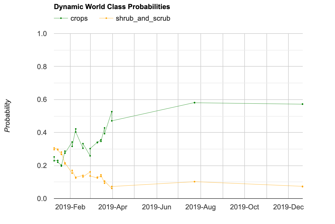
Dynamic World Time-Series
// Charting Class Probabilities Over Time

var geometry = ee.Geometry.Polygon([[
  [36.62513180012346, -1.2332928138897847],
  [36.62499232525469, -1.2339685738967323],
  [36.62524981732012, -1.234011479288199],
  [36.62541074986101, -1.2334322564449516]]
]);

Map.addLayer(geometry, {color: 'red'}, 'Selected Location')
Map.centerObject(geometry, 16)

// Filter the Dynamic World collection for the time period and
// location of interest.
var startDate = ee.Date.fromYMD(2019, 1, 1);
var endDate = startDate.advance(1, 'year');

var dw = ee.ImageCollection('GOOGLE/DYNAMICWORLD/V1')
  .filter(ee.Filter.date(startDate, endDate))
  .filter(ee.Filter.bounds(geometry))

var probabilityBands = [
    'water', 'trees', 'grass', 'flooded_vegetation', 'crops',
    'shrub_and_scrub', 'built', 'bare', 'snow_and_ice'
    ];

// Select all probability bands
var dwTimeSeries = dw.select(probabilityBands)

// Plot the time series for a single class
var chart = ui.Chart.image.series({
  imageCollection: dwTimeSeries.select('crops'),
  region: geometry,
  scale: 10
}).setOptions({
      lineWidth: 0.5,
      pointSize: 1,
      title: 'Dynamic World Class Probability (Crops)',
      interpolateNulls: true,
      vAxis: {title: 'Probability', viewWindow: {min:0, max:1}},
      hAxis: {title: '', format: 'YYYY-MMM'},
      series: {
        0: {color: 'green'}
      }
    })
print(chart)

// Plot the time series for a multiple classes

var chart = ui.Chart.image.series({
  imageCollection: dwTimeSeries.select(['crops', 'shrub_and_scrub']),
  region: geometry,
  scale: 10
}).setOptions({
      lineWidth: 0.5,
      pointSize: 1,
      title: 'Dynamic World Class Probabilities',
      interpolateNulls: true,
      vAxis: {title: 'Probability', viewWindow: {min:0, max:1}},
      hAxis: {title: '', format: 'YYYY-MMM'},
      series: {
        0: {color: 'green'},
        1: {color: 'orange'}
      },
      legend: {
        position: 'top'
      }
    });
print(chart);
Exercise
Quiz - Module 3
This is a short quiz to test your understanding of the Module 3 concepts.
Module 4: Earth Engine Apps
01. Client vs. Server
var date = '2020-01-01' // This is client-side
print(typeof(date))

var eedate = ee.Date('2020-01-01').format() // This is server-side
print(typeof(eedate))

// To bring server-side objects to client-side, you can call .getInfo()

// var clientdate = eedate.getInfo()
// print(clientdate)
// print(typeof(clientdate))

// getInfo() blocks the execution of your code till the value is fetched
// If the value takes time to compute, your code editor will freeze
// This is not a good user experience
var s2 = ee.ImageCollection("COPERNICUS/S2_SR")
var filtered = s2.filter(ee.Filter.date('2020-01-01', '2021-01-01'))

//var numImages = filtered.size().getInfo()
//print(numImages)

// A better approach is to use evaluate() function

// You need to define a 'callback' function which will be called once the
// value has been computed and ready to be used.

var myCallback = function(object) {
  print(object)
}
print('Computing the size of the collection')
var numImages = filtered.size().evaluate(myCallback)
Exercise
var date = ee.Date.fromYMD(2019, 1, 1)
print(date)

// We can use the format() function to create
// a string from a date object
var dateString = date.format('dd MMM, YYYY')
print(dateString)

// Exercise
// The print statement below combines a client-side string
// with a server-side string - resulting in an error.

// Fix the code so that the following message is printed
// 'The date is 01 Jan, 2019'
var message = 'The date is ' + dateString
print(message)

// Hint:
// Convert the client-side string to a server-side string
// Use ee.String() to create a server-side string
// Use the .cat() function instead of + to combine 2 strings
02. Using UI Elements
// You can add any widgets from the ui.* module to the map
var startYears = ['2017', '2018', '2019', '2020', '2021', '2022'];
var endYears = ['2018', '2019', '2020', '2021', '2022', '2023'];
// Let's create a ui.Select() dropdown with the above values
var startYearSelector = ui.Select({
  items: startYears,
  value: '2017',
  placeholder: 'Select start year',
  })
Map.add(startYearSelector);

var endYearSelector = ui.Select({
  items: endYears,
  value: '2023',
  placeholder: 'Select start year',
  })
Map.add(endYearSelector);

var probabilityBands = [
    'water', 'trees', 'grass', 'flooded_vegetation', 'crops',
    'shrub_and_scrub', 'built', 'bare', 'snow_and_ice'
    ];
var bandSelector = ui.Select({
  items: probabilityBands,
  value: 'built'
})
Map.add(bandSelector);


var loadImages = function() {

  var admin2 = ee.FeatureCollection('FAO/GAUL_SIMPLIFIED_500m/2015/level2');
  var kenyaAdmin2 = admin2.filter(ee.Filter.eq('ADM0_NAME', 'Kenya'));
  var geometry = kenyaAdmin2.geometry();

  var startYear = startYearSelector.getValue();
  var endYear = endYearSelector.getValue();
  var band = bandSelector.getValue();
  var beforeStart = ee.Date.fromYMD(ee.Number.parse(startYear), 1, 1);
  var beforeEnd = beforeStart.advance(1, 'year');

  var afterStart = ee.Date.fromYMD(ee.Number.parse(endYear), 1, 1);
  var afterEnd = afterStart.advance(1, 'year');

  var dw = ee.ImageCollection('GOOGLE/DYNAMICWORLD/V1')
    .select(band);

  var beforeDw = dw
    .filter(ee.Filter.date(beforeStart, beforeEnd))
    .mean();

  var afterDw = dw
    .filter(ee.Filter.date(afterStart, afterEnd))
    .mean();

  var probabilityVis = {min:0, max:1};
  Map.addLayer(beforeDw.clip(geometry), probabilityVis, 'Before Probability');
  Map.addLayer(afterDw.clip(geometry), probabilityVis, 'After Probability');
};

var button = ui.Button({
  label: 'Click to Load Images',
  onClick: loadImages,
  });
Map.add(button);
Exercise
// Instead of manually creating a list of years like before
// we can create a list of years using ee.List.sequence()
var years = ee.List.sequence(2017, 2023)

// Convert them to strings using format() function
var yearStrings = years.map(function(year){
  return ee.Number(year).format('%04d')
})
print(yearStrings);

// Convert the server-side object to client-side using
// evaluate() and use it with ui.Select()
yearStrings.evaluate(function(yearList) {
  var yearSelector = ui.Select({
    items: yearList,
    value: '2017',
    placeholder: 'Select a year',
    })
  Map.add(yearSelector)
});

// Exercise

// Create another dropdown with months from 1 to 12
// and add it to the map.
03. Building a Change Detection App
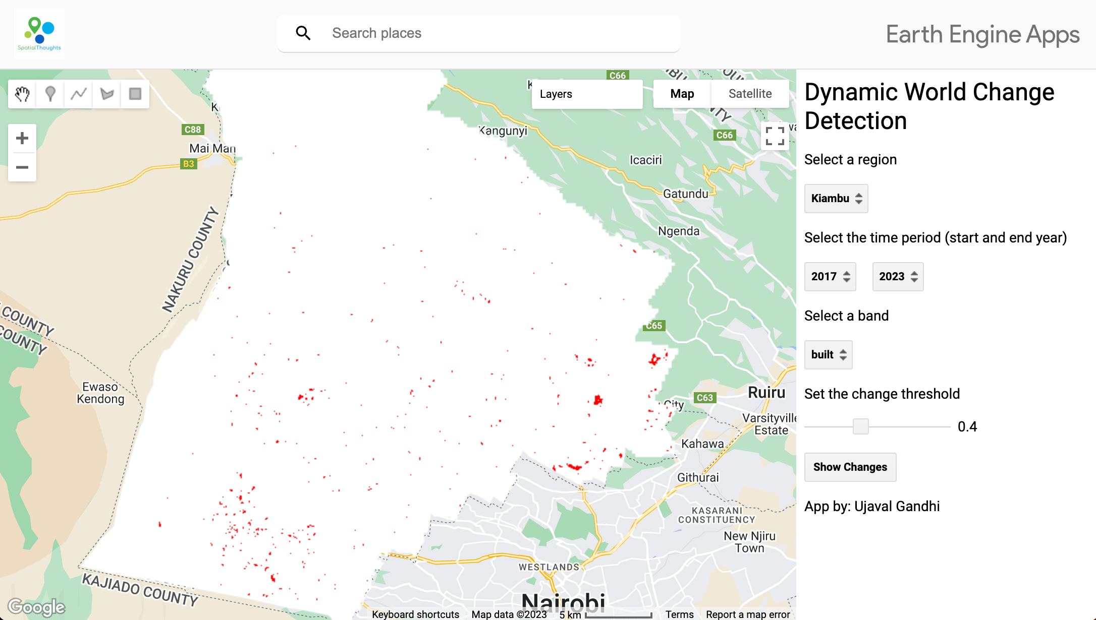
// Panels are the main container widgets
var mainPanel = ui.Panel({
  style: {width: '300px'}
});


var title = ui.Label({
  value: 'Dynamic World Change Detection',
  style: {'fontSize': '24px'}
});
// You can add widgets to the panel
mainPanel.add(title);

var adminLabel = ui.Label('Select a region');
mainPanel.add(adminLabel);
// You can even add panels to other panels
var adminPanel = ui.Panel({
  layout: ui.Panel.Layout.flow('horizontal'),
});
mainPanel.add(adminPanel);

var adminSelector = ui.Select();
adminPanel.add(adminSelector);

var yearLabel = ui.Label('Select the time period (start and end year)');
mainPanel.add(yearLabel);
var yearPanel = ui.Panel({
  layout: ui.Panel.Layout.flow('horizontal'),
});
mainPanel.add(yearPanel);

var startYearSelector = ui.Select();

var endYearSelector = ui.Select();


yearPanel.add(startYearSelector);
yearPanel.add(endYearSelector);

var bandPanel = ui.Panel({
  layout: ui.Panel.Layout.flow('horizontal'),
});
var probabilityBands = [
    'water', 'trees', 'grass', 'flooded_vegetation', 'crops',
    'shrub_and_scrub', 'built', 'bare', 'snow_and_ice'
    ];
var bandLabel = ui.Label('Select a band');
mainPanel.add(bandLabel);

var bandSelector = ui.Select({
  items: probabilityBands,
  value: 'built'
  });
bandPanel.add(bandSelector);
mainPanel.add(bandPanel);


var thresholdLabel = ui.Label('Set the change threshold');
mainPanel.add(thresholdLabel);
var thresholdPanel = ui.Panel({
  layout: ui.Panel.Layout.flow('horizontal'),
    style: {width: '250px'}

});
mainPanel.add(thresholdPanel);

var slider = ui.Slider({
  min: 0.1,
  max: 0.9,
  value: 0.5,
  step: 0.1,
  style: {width: '200px'}

});
thresholdPanel.add(slider);

var button = ui.Button('Show Changes');
mainPanel.add(button);

// Let's add a dropdown with all admin2 areas
var admin2 = ee.FeatureCollection('FAO/GAUL_SIMPLIFIED_500m/2015/level2');

var kenyaAdmin2 = admin2.filter(ee.Filter.eq('ADM0_NAME', 'Kenya'));
var kenyaAdmin2Names = kenyaAdmin2.aggregate_array('ADM2_NAME');

// Evaluate the results and populate the dropdown
kenyaAdmin2Names.evaluate(function(kenyaAdmin2NamesList) {
  adminSelector.items().reset(kenyaAdmin2NamesList);
    adminSelector.setValue(kenyaAdmin2NamesList[0]);
});

// Let's add dropdown with start and end years
var startYears = ee.List.sequence(2017, 2023);
var endYears = ee.List.sequence(2018, 2023);

// Dropdown items need to be strings
var startYearsStrings = startYears.map(function(year){
  return ee.Number(year).format('%04d');
});

var endYearsStrings = endYears.map(function(year){
  return ee.Number(year).format('%04d');
});

// Evaluate the results and populate the dropdown
startYearsStrings.evaluate(function(yearList) {
  startYearSelector.items().reset(yearList);
  startYearSelector.setValue(yearList[0]);
});

endYearsStrings.evaluate(function(yearList) {
  endYearSelector.items().reset(yearList);
  endYearSelector.setValue(yearList[yearList.length -1]);
});


// Define a function that triggers when any value is changed
var showChange = function() {
  var startYear = startYearSelector.getValue();
  var endYear = endYearSelector.getValue();
  var band = bandSelector.getValue();
  var threshold = slider.getValue();
  var admin2Value = adminSelector.getValue();

  var selectedAdmin2 = admin2.filter(ee.Filter.eq('ADM2_NAME', admin2Value));
  var geometry = selectedAdmin2.geometry();

  var beforeStart = ee.Date.fromYMD(ee.Number.parse(startYear), 1, 1);
  var beforeEnd = beforeStart.advance(1, 'year');

  var afterStart = ee.Date.fromYMD(ee.Number.parse(endYear), 1, 1);
  var afterEnd = afterStart.advance(1, 'year');

  var dw = ee.ImageCollection('GOOGLE/DYNAMICWORLD/V1')
  .filterBounds(geometry).select(band);

  var beforeDw = dw
    .filter(ee.Filter.date(beforeStart, beforeEnd))
    .mean();

  var afterDw = dw
    .filter(ee.Filter.date(afterStart, afterEnd))
    .mean();

  var diff = afterDw.subtract(beforeDw);
  var change = diff.abs().gt(threshold);

  var changeVisParams = {min: 0, max: 1, palette: ['white', 'red']};
  Map.centerObject(geometry);
  Map.addLayer(change.clip(geometry), changeVisParams, 'Change');
};
button.onClick(showChange);

Map.setCenter(37.794, 0.341, 7);

ui.root.add(mainPanel);
Exercise
04. Publishing the App
// Panels are the main container widgets
var mainPanel = ui.Panel({
  style: {width: '300px'}
});


var title = ui.Label({
  value: 'Dynamic World Change Detection',
  style: {'fontSize': '24px'}
});
// You can add widgets to the panel
mainPanel.add(title);

var adminLabel = ui.Label('Select a region');
mainPanel.add(adminLabel);
// You can even add panels to other panels
var adminPanel = ui.Panel({
  layout: ui.Panel.Layout.flow('horizontal'),
});
mainPanel.add(adminPanel);

var adminSelector = ui.Select();
adminPanel.add(adminSelector);

var yearLabel = ui.Label('Select the time period (start and end year)');
mainPanel.add(yearLabel);
var yearPanel = ui.Panel({
  layout: ui.Panel.Layout.flow('horizontal'),
});
mainPanel.add(yearPanel);

var startYearSelector = ui.Select();

var endYearSelector = ui.Select();


yearPanel.add(startYearSelector);
yearPanel.add(endYearSelector);

var bandPanel = ui.Panel({
  layout: ui.Panel.Layout.flow('horizontal'),
});
var probabilityBands = [
    'water', 'trees', 'grass', 'flooded_vegetation', 'crops',
    'shrub_and_scrub', 'built', 'bare', 'snow_and_ice'
    ];
var bandLabel = ui.Label('Select a band');
mainPanel.add(bandLabel);

var bandSelector = ui.Select({
  items: probabilityBands,
  value: 'built'
  });
bandPanel.add(bandSelector);
mainPanel.add(bandPanel);


var thresholdLabel = ui.Label('Set the change threshold');
mainPanel.add(thresholdLabel);
var thresholdPanel = ui.Panel({
  layout: ui.Panel.Layout.flow('horizontal'),
    style: {width: '250px'}

});
mainPanel.add(thresholdPanel);

var slider = ui.Slider({
  min: 0.1,
  max: 0.9,
  value: 0.5,
  step: 0.1,
  style: {width: '200px'}

});
thresholdPanel.add(slider);

var button = ui.Button('Show Changes');
mainPanel.add(button);

// Let's add a dropdown with all admin2 areas
var admin2 = ee.FeatureCollection('FAO/GAUL_SIMPLIFIED_500m/2015/level2');

var kenyaAdmin2 = admin2.filter(ee.Filter.eq('ADM0_NAME', 'Kenya'));
var kenyaAdmin2Names = kenyaAdmin2.aggregate_array('ADM2_NAME');

// Evaluate the results and populate the dropdown
kenyaAdmin2Names.evaluate(function(kenyaAdmin2NamesList) {
  adminSelector.items().reset(kenyaAdmin2NamesList);
    adminSelector.setValue(kenyaAdmin2NamesList[0]);
});

// Let's add dropdown with start and end years
var startYears = ee.List.sequence(2017, 2023);
var endYears = ee.List.sequence(2018, 2023);

// Dropdown items need to be strings
var startYearsStrings = startYears.map(function(year){
  return ee.Number(year).format('%04d');
});

var endYearsStrings = endYears.map(function(year){
  return ee.Number(year).format('%04d');
});

// Evaluate the results and populate the dropdown
startYearsStrings.evaluate(function(yearList) {
  startYearSelector.items().reset(yearList);
  startYearSelector.setValue(yearList[0]);
});

endYearsStrings.evaluate(function(yearList) {
  endYearSelector.items().reset(yearList);
  endYearSelector.setValue(yearList[yearList.length -1]);
});


// Define a function that triggers when any value is changed
var showChange = function() {
  var startYear = startYearSelector.getValue();
  var endYear = endYearSelector.getValue();
  var band = bandSelector.getValue();
  var threshold = slider.getValue();
  var admin2Value = adminSelector.getValue();

  var selectedAdmin2 = admin2.filter(ee.Filter.eq('ADM2_NAME', admin2Value));
  var geometry = selectedAdmin2.geometry();

  var beforeStart = ee.Date.fromYMD(ee.Number.parse(startYear), 1, 1);
  var beforeEnd = beforeStart.advance(1, 'year');

  var afterStart = ee.Date.fromYMD(ee.Number.parse(endYear), 1, 1);
  var afterEnd = afterStart.advance(1, 'year');

  var dw = ee.ImageCollection('GOOGLE/DYNAMICWORLD/V1')
  .filterBounds(geometry).select(band);

  var beforeDw = dw
    .filter(ee.Filter.date(beforeStart, beforeEnd))
    .mean();

  var afterDw = dw
    .filter(ee.Filter.date(afterStart, afterEnd))
    .mean();

  var diff = afterDw.subtract(beforeDw);
  var change = diff.abs().gt(threshold);

  var changeVisParams = {min: 0, max: 1, palette: ['white', 'red']};
  Map.clear();
  Map.centerObject(geometry);
  Map.addLayer(change.clip(geometry), changeVisParams, 'Change');
};
button.onClick(showChange);


var authorLabel = ui.Label('App by: Ujaval Gandhi');
mainPanel.add(authorLabel);

Map.setCenter(37.794, 0.341, 7);

ui.root.add(mainPanel);
Exercise
05. Split-Panel App
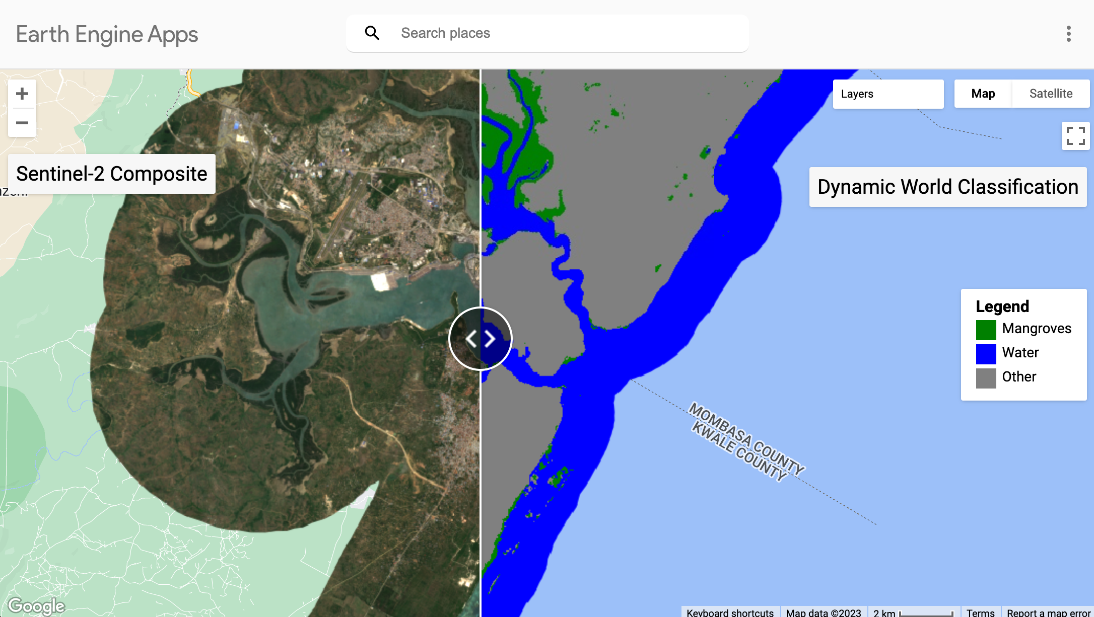
var compositeS2 = ee.Image('users/ujavalgandhi/kenya/mangroves_composite');
var classifiedDw = ee.Image('users/ujavalgandhi/kenya/mangroves_classified_dw');


// Create a Split Panel App

// Set a center and zoom level.
var center = {lon: 39.67, lat: -4.069, zoom: 12};

// Create two maps.
var leftMap = ui.Map(center);
var rightMap = ui.Map(center);

// Link them together.
var linker = new ui.Map.Linker([leftMap, rightMap]);

// Create a split panel with the two maps.
var splitPanel = ui.SplitPanel({
  firstPanel: leftMap,
  secondPanel: rightMap,
  orientation: 'horizontal',
  wipe: true
});

// Remove the default map from the root panel.
ui.root.clear();

// Add our split panel to the root panel.
ui.root.add(splitPanel);

// Add the layers to the maps
var classVis = {min:1, max:3, palette: ['green', 'blue', 'gray']};
var rgbVis = {min: 0, max: 0.3, bands: ['B4', 'B3', 'B2']};

// S2 classification goes to the leftMap
leftMap.addLayer(compositeS2, rgbVis, 'S2 Composite');

// Dynamic World Classification goes to the rightMap
rightMap.addLayer(classifiedDw, classVis, 'Dw Classified');

// We can also add a legend
var legend = ui.Panel({style: {position: 'middle-right', padding: '8px 15px'}});

var makeRow = function(color, name) {
  var colorBox = ui.Label({
    style: {color: '#ffffff',
      backgroundColor: color,
      padding: '10px',
      margin: '0 0 4px 0',
    }
  });
  var description = ui.Label({
    value: name,
    style: {
      margin: '0px 0 4px 6px',
    }
  });
  return ui.Panel({
    widgets: [colorBox, description],
    layout: ui.Panel.Layout.Flow('horizontal')}
)};

var title = ui.Label({
  value: 'Legend',
  style: {fontWeight: 'bold',
    fontSize: '16px',
    margin: '0px 0 4px 0px'}});

legend.add(title);
legend.add(makeRow('green','Mangroves'));
legend.add(makeRow('blue','Water'));
legend.add(makeRow('gray','Other'));

rightMap.add(legend);
Exercise
// Add the following labels to the appropriate map
var label1 = ui.Label({value: 'Sentinel-2 Composite',
  style: {'fontSize': '20px', backgroundColor: '#f7f7f7', position:'top-left'}});
var label2 = ui.Label({value: 'Dynamic World Classification',
  style: {'fontSize': '20px', backgroundColor: '#f7f7f7', position:'top-right'}});
Supplement
Automated GCP Collection for Mangrove Classification
// Script to preare Coastline AOI and Training Samples
// for mangrove classification

// Prepare a Coastline Buffer Geometry

// Using LSIB for country boundaries
var lsib = ee.FeatureCollection('USDOS/LSIB_SIMPLE/2017');

// Select a country and change the 'aoi' variable below
// to be a rectangle covering the coastline of the chosen country.
var country = 'Kenya';
var selected = lsib.filter(ee.Filter.eq('country_na', country));
var geometry = selected.geometry();

// Draw a bounding box covering the coastline
var aoi = ee.Geometry.Polygon([[
  [39.19974759779212, -1.6713255840099857],
  [39.19974759779212, -4.691668023633792],
  [41.638787348385165, -4.691668023633792],
  [41.638787348385165, -1.6713255840099857]
]]);

// Define the distance in meters
var landDistance = 5000;
var oceanDistance = 2000;

// Buffer each polygon inwards by the distance and compute the difference
// The result will be a buffer region for the entire polygon
var buffer1 = geometry.symmetricDifference(geometry.buffer(oceanDistance));
var buffer2 = geometry.symmetricDifference(geometry.buffer(-1*landDistance));

// Put both in a collection
var result = ee.FeatureCollection([buffer1, buffer2]);

var coastline = result.geometry().dissolve({maxError:100});

var geometry = coastline.intersection({
  right: aoi,
  maxError: 100});
Map.addLayer(geometry)

var coastlineFc = ee.FeatureCollection([
  ee.Feature(geometry, {
    'land_distance': landDistance,
    'ocean_distance': oceanDistance
  })
]);

Export.table.toAsset({
  collection: coastlineFc,
  description: 'Coastline',
  assetId: 'users/ujavalgandhi/kenya/kenya_coastline'
});

// Prepare Trainin Samples

// Use Global Mangrove Watch Dataset
// for sampling mangrove GCPs
var mangrovesVector = ee.FeatureCollection(
  'projects/earthengine-legacy/assets/projects/sat-io/open-datasets/GMW/extent/gmw_v3_2020_vec');
Map.addLayer(mangrovesVector, {color:'gray'}, 'Mangroves (vector)', false)

var mangroveRaster = mangrovesVector.reduceToImage({
  properties: ['PXLVAL'],
  reducer: ee.Reducer.first()
});
var mangroveRaster = mangroveRaster.rename('landcover');
var classVis = {min:0, max:1, palette: ['white', 'green']}

Map.addLayer(mangroveRaster.clip(geometry), classVis, 'Mangroves Original', false)

// Use Global Surface Water Dataset
// for sampling water GCPs
var gswYearly = ee.ImageCollection('JRC/GSW1_4/YearlyHistory');

var filtered = gswYearly.filter(ee.Filter.eq('year', 2020))
var gsw2020 = ee.Image(filtered.first())

// Select permanent water
var water = gsw2020.eq(3)
var waterVis = {min:0, max:1, palette: ['white', 'blue']}

Map.addLayer(water.clip(geometry), waterVis, 'Water Original', false)

// Combine both images to create a 3 class image

var classified = ee.Image(3)
  .where(mangroveRaster.eq(1), 1)
  .where(water.eq(1), 2)
  .rename('landcover')

var classVis = {min:1, max:3, palette: ['green', 'blue', 'gray']}

Map.addLayer(classified.clip(geometry),classVis, 'Classified' )

var mangroves = classified.eq(1);
var water = classified.eq(2);
var other = classified.eq(3);

// Perform a dilation to identify core areas.
// This avoids samples from the edges
var processImage = function(image) {
  var imageProcessed = image.focalMin({
    radius: 10,
    kernelType: 'circle',
    units: 'meters',
    iterations: 1});
  return imageProcessed;
};

// Apply processing
var mangrovesProcessed = processImage(mangroves);
var waterProcessed = processImage(water);
var otherProcessed = processImage(other);


// Combine all images
var processedImage = mangrovesProcessed
  .add(waterProcessed.multiply(2))
  .add(otherProcessed.multiply(3))
  .selfMask()


Map.addLayer(processedImage.clip(geometry), classVis, 'Core areas to sample' );

// Sample points
var gcps = processedImage.stratifiedSample({
  numPoints: 250,
  classBand: 'landcover',
  region: geometry,
  scale: 10,
  geometries: true,
  dropNulls: true
});
Map.addLayer(gcps, {color: 'yellow'}, 'Samples', false);

Export.table.toAsset({
  collection: gcps,
  description: 'Samples',
  assetId: 'users/ujavalgandhi/kenya/mangroves_gcps'});
Learning Resources
- Google Earth Engine User Guide
- Cloud-Based Remote Sensing with Google Earth Engine: Fundamentals and Applications: A free and open-access book with 55-chapters covering fundamentals and applications of GEE. Also includes YouTube videos summarizing each chapter.
- Spatial Thoughts
OpenCourseWare
- End-to-End Google Earth Engine
- Google Earth Engine for Water Resources Management
- Creating Publication Quality Charts with GEE
- Earth Engine Advanced Concepts
Data Credits
- Sentinel-2 Level-1C, Level-2A and Sentinel-1 SAR GRD: Contains Copernicus Sentinel data.
- Dynamic World V1: Brown, C.F., Brumby, S.P., Guzder-Williams, B. et al. Dynamic World, Near real-time global 10 m land use land cover mapping. Sci Data 9, 251 (2022). doi:10.1038/s41597-022-01307-4
- Kenya Admin Level 4 boundaries: Central Bureau of Statistics (CBS), OCHA Regional Office for Southern and Eastern Africa (ROSEA). Downloaded from https://data.humdata.org/dataset/kenya-admin-level-4-boundaries
- LSIB 2017: Large Scale International Boundary Polygons, Simplified: United States Department of State, Office of the Geographer
- FAO GAUL 500m: Global Administrative Unit Layers 2015, Second-Level Administrative Units: Source of Administrative boundaries: The Global Administrative Unit Layers (GAUL) dataset, implemented by FAO within the CountrySTAT and Agricultural Market Information System (AMIS) projects.
License
The course material (text, images, presentation, videos) is licensed under a Creative Commons Attribution 4.0 International License.
The code (scripts, Jupyter notebooks) is licensed under the MIT License. For a copy, see https://opensource.org/licenses/MIT
Kindly give appropriate credit to the original author as below:
Copyright © 2023 Ujaval Gandhi www.spatialthoughts.com
Citing and Referencing
You can cite the course materials as follows
- Gandhi, Ujaval, 2023. Hands-on Introduction to Dynamic World workshop. Spatial Thoughts. https://courses.spatialthoughts.com/gee-dynamic-world.html
If you want to report any issues with this page, please comment below.