Introduction

This 5-hour hands-on workshop is designed to help participants learn the basics of the Google Earth Engine platform. This beginner-friendly class covers a range of topics to help participants get comfortable with the Code Editor environment and the Google Earth Engine API to implement remote sensing workflows. During the workshop, you will learn how to load, filter, analyze, and export datasets from the Earth Engine Data Catalog. The workshop also covers Map/Reduce programming concepts so you can scale your analysis to large regions and work with time-series data.

Pre-requisites:

Familiarity with remote sensing datasets and concepts is helpful but not required.
No programming background or experience is required.

View the Presentation ↗

Setting up the Environment

Get the Course Materials

The course material and exercises are in the form of Earth Engine scripts shared via a code repository.

Click this link to open Google Earth Engine code editor and add the repository to your account.
If successful, you will have a new repository named users/ujavalgandhi/GEE-Introduction in the Scripts tab in the Reader section.
Verify that your code editor looks like below

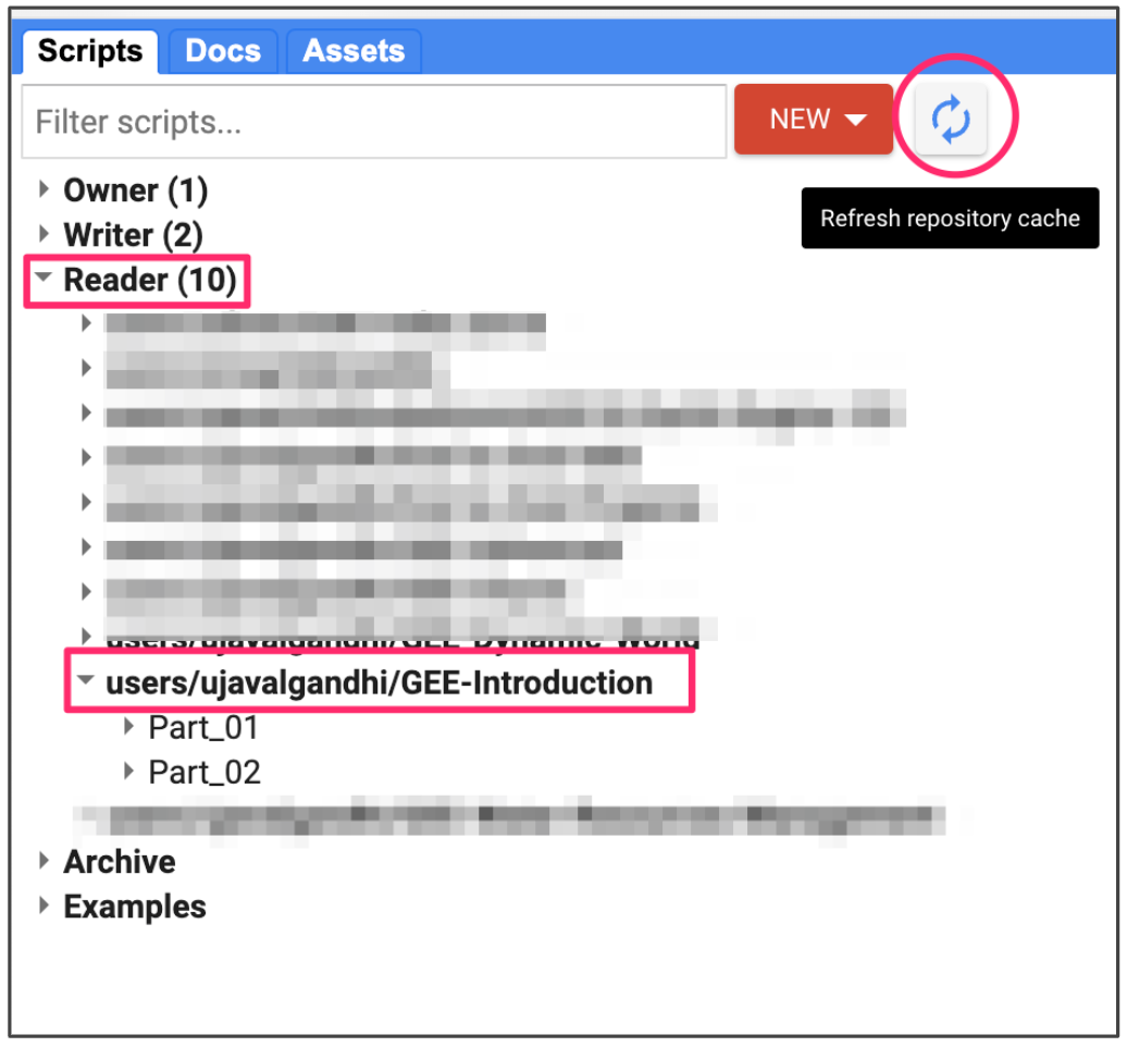
Code Editor After Adding the Workshop Repository

If you do not see the repository in the Reader section, click Refresh repository cache button in your Scripts tab and it will show up.

Get the Course Videos

The course is accompanied by a set of professionally edited videos recorded during Geo For Good 2023 conference and available via the Google Earth YouTube channel. Access the YouTube Playlist ↗

Part 1: Data Discovery, Processing and Export

01. Hello World

Open in Code Editor ↗

print('Hello World');

// Variables
var city = 'Bengaluru';
var country = 'India';
print(city, country);

var population = 8400000;
print(population);
 
// List
var majorCities = ['Mumbai', 'Delhi', 'Chennai', 'Kolkata'];
print(majorCities);

// Dictionary
var cityData = {
  'city': city,
  'population': 8400000,
  'elevation': 930
};
print(cityData);

// Function
var greet = function(name) {
    return 'Hello ' + name;
};
print(greet('World'));

// This is a comment

Exercise

Try in Code Editor ↗

// These are the 5 largest cities in the world: 
// Tokyo, Delhi, Shanghai, Mexico City, Sao Paulo

// Create a list named 'largeCities'
// The list should have names of all the above cities
// Print the list

02. ImageCollections

Open in Code Editor ↗

/**
 * Function to mask clouds using the Sentinel-2 QA band
 * @param {ee.Image} image Sentinel-2 image
 * @return {ee.Image} cloud masked Sentinel-2 image
 */
function maskS2clouds(image) {
  var qa = image.select('QA60');

  // Bits 10 and 11 are clouds and cirrus, respectively.
  var cloudBitMask = 1 << 10;
  var cirrusBitMask = 1 << 11;

  // Both flags should be set to zero, indicating clear conditions.
  var mask = qa.bitwiseAnd(cloudBitMask).eq(0)
      .and(qa.bitwiseAnd(cirrusBitMask).eq(0));

  return image.updateMask(mask).divide(10000);
}

// Map the function over a month of data and take the median.
// Load Sentinel-2 TOA reflectance data (adjusted for processing changes
// that occurred after 2022-01-25).
var dataset = ee.ImageCollection('COPERNICUS/S2_HARMONIZED')
                  .filterDate('2022-01-01', '2022-01-31')
                  // Pre-filter to get less cloudy granules.
                  .filter(ee.Filter.lt('CLOUDY_PIXEL_PERCENTAGE', 20))
                  .map(maskS2clouds);

var rgbVis = {
  min: 0.0,
  max: 0.3,
  bands: ['B4', 'B3', 'B2'],
};

Map.setCenter(-9.1695, 38.6917, 12);
Map.addLayer(dataset.median(), rgbVis, 'RGB');

Exercise

Try in Code Editor ↗

// Exercise

// Find the 'Sentinel-2 Level-1C' dataset page
// https://developers.google.com/earth-engine/datasets

// Copy/paste the code snippet

// Change the code to display images for your home city

03. Filtering ImageCollections

Open in Code Editor ↗

/**** Start of imports. If edited, may not auto-convert in the playground. ****/
var geometry = /* color: #d63000 */ee.Geometry.Point([77.60412933051538, 12.952912912328241]);
/***** End of imports. If edited, may not auto-convert in the playground. *****/
Map.centerObject(geometry, 10)

var s2 = ee.ImageCollection('COPERNICUS/S2_HARMONIZED');

// Filter by metadata
var filtered = s2.filter(ee.Filter.lt('CLOUDY_PIXEL_PERCENTAGE', 30));

// Filter by date
var filtered = s2.filter(ee.Filter.date('2019-01-01', '2020-01-01'));

// Filter by location
var filtered = s2.filter(ee.Filter.bounds(geometry));

// Let's apply all the 3 filters together on the collection

// First apply metadata fileter
var filtered1 = s2.filter(ee.Filter.lt('CLOUDY_PIXEL_PERCENTAGE', 30));
// Apply date filter on the results
var filtered2 = filtered1.filter(
  ee.Filter.date('2019-01-01', '2020-01-01'));
// Lastly apply the location filter
var filtered3 = filtered2.filter(ee.Filter.bounds(geometry));

// Instead of applying filters one after the other, we can 'chain' them
// Use the . notation to apply all the filters together
var filtered = s2
  .filter(ee.Filter.lt('CLOUDY_PIXEL_PERCENTAGE', 30))
  .filter(ee.Filter.date('2019-01-01', '2020-01-01'))
  .filter(ee.Filter.bounds(geometry));
  
print(filtered.size());

Exercise

Try in Code Editor ↗

/**** Start of imports. If edited, may not auto-convert in the playground. ****/
var geometry = /* color: #98ff00 */ee.Geometry.Point([77.60412933051538, 12.952912912328241]);
/***** End of imports. If edited, may not auto-convert in the playground. *****/
Map.centerObject(geometry, 10);

var s2 = ee.ImageCollection('COPERNICUS/S2_HARMONIZED');

var filtered = s2
  .filter(ee.Filter.lt('CLOUDY_PIXEL_PERCENTAGE', 30))
  .filter(ee.Filter.date('2019-01-01', '2020-01-01'))
  .filter(ee.Filter.bounds(geometry));

print(filtered.size());

// Exercise
// Delete the 'geometry' import
// Add a point at your chosen location
// Change the filter to find images from September 2023

04. Mosaics and Composites

Open in Code Editor ↗

/**** Start of imports. If edited, may not auto-convert in the playground. ****/
var geometry = /* color: #0B4A8B */ee.Geometry.Point([77.60412933051538, 12.952912912328241]);
/***** End of imports. If edited, may not auto-convert in the playground. *****/
var s2 = ee.ImageCollection('COPERNICUS/S2_HARMONIZED');

var rgbVis = {
  min: 0.0,
  max: 3000,
  bands: ['B4', 'B3', 'B2'],
};
var filtered = s2.filter(ee.Filter.lt('CLOUDY_PIXEL_PERCENTAGE', 30))
  .filter(ee.Filter.date('2019-01-01', '2020-01-01'))
  .filter(ee.Filter.bounds(geometry));
 
var mosaic = filtered.mosaic();
 
var medianComposite = filtered.median();

Map.addLayer(filtered, rgbVis, 'Filtered Collection');
Map.addLayer(mosaic, rgbVis, 'Mosaic');
Map.addLayer(medianComposite, rgbVis, 'Median Composite');

Exercise

Try in Code Editor ↗

/**** Start of imports. If edited, may not auto-convert in the playground. ****/
var geometry = /* color: #ffc82d */ee.Geometry.Point([77.60412933051538, 12.952912912328241]);
/***** End of imports. If edited, may not auto-convert in the playground. *****/
Map.centerObject(geometry, 10);
var s2 = ee.ImageCollection('COPERNICUS/S2_HARMONIZED');

var rgbVis = {
  min: 0.0,
  max: 3000,
  bands: ['B4', 'B3', 'B2'], 
};
var filtered = s2.filter(ee.Filter.lt('CLOUDY_PIXEL_PERCENTAGE', 30))
  .filter(ee.Filter.date('2019-01-01', '2020-01-01'))
  .filter(ee.Filter.bounds(geometry));

var image2019 = filtered.median();
Map.addLayer(image2019, rgbVis, '2019');

// Exercise
// Delete the 'geometry' import
// Add a point at your chosen location
// Create a median composite for both 2019 and 2020
// Display both on the map

05. FeatureCollections

Open in Code Editor ↗

/**** Start of imports. If edited, may not auto-convert in the playground. ****/
var admin2 = ee.FeatureCollection("FAO/GAUL_SIMPLIFIED_500m/2015/level2");
/***** End of imports. If edited, may not auto-convert in the playground. *****/
var filtered = admin2
  .filter(ee.Filter.eq('ADM1_NAME', 'Karnataka'))
  .filter(ee.Filter.eq('ADM2_NAME', 'Bangalore Urban'));

Map.centerObject(filtered)

Map.addLayer(filtered, {'color': 'red'}, 'Selected Admin2');

Exercise

Try in Code Editor ↗

/**** Start of imports. If edited, may not auto-convert in the playground. ****/
var admin2 = ee.FeatureCollection("FAO/GAUL_SIMPLIFIED_500m/2015/level2");
/***** End of imports. If edited, may not auto-convert in the playground. *****/
Map.addLayer(admin2, {}, 'All Admin2');

// Exercise

// Inspect and find the name of ADM1_NAME and ADM2_NAME properties
// of your chosen Admin2 region

// Apply filters and display the chosen Admin2 region in 'blue' color

06. Clipping

Open in Code Editor ↗

/**** Start of imports. If edited, may not auto-convert in the playground. ****/
var s2 = ee.ImageCollection("COPERNICUS/S2_HARMONIZED"),
    admin2 = ee.FeatureCollection("FAO/GAUL_SIMPLIFIED_500m/2015/level2");
/***** End of imports. If edited, may not auto-convert in the playground. *****/
var filteredAdmin2 = admin2
  .filter(ee.Filter.eq('ADM1_NAME', 'Karnataka'))
  .filter(ee.Filter.eq('ADM2_NAME', 'Bangalore Urban'));

var geometry = filteredAdmin2.geometry();

var filteredS2 = s2.filter(ee.Filter.lt('CLOUDY_PIXEL_PERCENTAGE', 30))
  .filter(ee.Filter.date('2019-01-01', '2020-01-01'))
  .filter(ee.Filter.bounds(geometry));

var image = filteredS2.median(); 

var clipped = image.clip(geometry);

var rgbVis = {
  min: 0.0,
  max: 3000,
  bands: ['B4', 'B3', 'B2'], 
};
Map.centerObject(geometry);
Map.addLayer(clipped, rgbVis, 'Clipped Composite');

Exercise

Try in Code Editor ↗

/**** Start of imports. If edited, may not auto-convert in the playground. ****/
var s2 = ee.ImageCollection("COPERNICUS/S2_HARMONIZED"),
    admin2 = ee.FeatureCollection("FAO/GAUL_SIMPLIFIED_500m/2015/level2");
/***** End of imports. If edited, may not auto-convert in the playground. *****/
var filteredAdmin2 = admin2
  .filter(ee.Filter.eq('ADM1_NAME', 'Karnataka'))
  .filter(ee.Filter.eq('ADM2_NAME', 'Bangalore Urban'));

var geometry = filteredAdmin2.geometry();

var filteredS2 = s2.filter(ee.Filter.lt('CLOUDY_PIXEL_PERCENTAGE', 30))
  .filter(ee.Filter.date('2019-01-01', '2020-01-01'))
  .filter(ee.Filter.bounds(geometry));

var image = filteredS2.median(); 

var clipped = image.clip(geometry);

var rgbVis = {
  min: 0.0,
  max: 3000,
  bands: ['B4', 'B3', 'B2'], 
};
Map.centerObject(geometry)
Map.addLayer(clipped, rgbVis, 'Clipped Composite');

// Exercise
// Change the filters to select the Admin2 region of your choice
// Display the clipped composite

07. Export

Open in Code Editor ↗

/**** Start of imports. If edited, may not auto-convert in the playground. ****/
var s2 = ee.ImageCollection("COPERNICUS/S2_HARMONIZED"),
    admin2 = ee.FeatureCollection("FAO/GAUL_SIMPLIFIED_500m/2015/level2");
/***** End of imports. If edited, may not auto-convert in the playground. *****/
var filteredAdmin2 = admin2
  .filter(ee.Filter.eq('ADM1_NAME', 'Karnataka'))
  .filter(ee.Filter.eq('ADM2_NAME', 'Bangalore Urban'));

var geometry = filteredAdmin2.geometry();

var filteredS2 = s2.filter(ee.Filter.lt('CLOUDY_PIXEL_PERCENTAGE', 30))
  .filter(ee.Filter.date('2019-01-01', '2020-01-01'))
  .filter(ee.Filter.bounds(geometry));

var image = filteredS2.median(); 

var clipped = image.clip(geometry);

var rgbVis = {
  min: 0.0,
  max: 3000,
  bands: ['B4', 'B3', 'B2'], 
};
Map.centerObject(geometry)
Map.addLayer(clipped, rgbVis, 'Clipped Composite');

var exportImage = clipped.select(['B4', 'B3', 'B2']);

Export.image.toDrive({
    image: exportImage,
    description: 'S2_Composite_Raw',
    folder: 'earthengine',
    fileNamePrefix: 's2_composite_raw',
    region: geometry,
    scale: 10,
    maxPixels: 1e9
});

// Rather than exporting raw bands, we can apply a rendered image
// visualize() function allows you to apply the same parameters 
// that are used in earth engine which exports a 3-band RGB image
print(clipped);
var visualized = clipped.visualize(rgbVis);
print(visualized);
// Now the 'visualized' image is RGB image, no need to give visParams
Map.addLayer(visualized, {}, 'Visualized Image');

Export.image.toDrive({
    image: visualized,
    description: 'S2_Composite_Visualized',
    folder: 'earthengine',
    fileNamePrefix: 'bs2_composite_visualized',
    region: geometry,
    scale: 10,
    maxPixels: 1e9
});

Exercise

Try in Code Editor ↗

/**** Start of imports. If edited, may not auto-convert in the playground. ****/
var s2 = ee.ImageCollection("COPERNICUS/S2_HARMONIZED"),
    admin2 = ee.FeatureCollection("FAO/GAUL_SIMPLIFIED_500m/2015/level2");
/***** End of imports. If edited, may not auto-convert in the playground. *****/
var filteredAdmin2 = admin2
  .filter(ee.Filter.eq('ADM1_NAME', 'Karnataka'))
  .filter(ee.Filter.eq('ADM2_NAME', 'Bangalore Urban'));

var geometry = filteredAdmin2.geometry();

var filteredS2 = s2.filter(ee.Filter.lt('CLOUDY_PIXEL_PERCENTAGE', 30))
  .filter(ee.Filter.date('2019-01-01', '2020-01-01'))
  .filter(ee.Filter.bounds(geometry));

var image = filteredS2.median(); 

var clipped = image.clip(geometry);

var rgbVis = {
  min: 0.0,
  max: 3000,
  bands: ['B4', 'B3', 'B2'], 
};
Map.centerObject(geometry)
Map.addLayer(clipped, rgbVis, 'Clipped Composite');

var exportImage = clipped.select(['B4', 'B3', 'B2']);

Export.image.toDrive({
    image: exportImage,
    description: 'S2_Composite',
    folder: 'earthengine',
    fileNamePrefix: 's2_composite',
    region: geometry,
    scale: 10,
    maxPixels: 1e9
});

// Exercise
// Change the filters to select the Admin2 region of your choice
// Export the composite image

Quiz 1

Take the short online quiz to recap your understanding of Part-1 of the workshop.

Launch Quiz-1 ↗.

Part 2: Computation in Earth Engine

01. Calculating Indices

Open in Code Editor ↗

/**** Start of imports. If edited, may not auto-convert in the playground. ****/
var s2 = ee.ImageCollection("COPERNICUS/S2_HARMONIZED"),
    geometry = /* color: #d63000 */ee.Geometry.Point([77.60412933051538, 12.952912912328241]);
/***** End of imports. If edited, may not auto-convert in the playground. *****/
var filteredS2 = s2.filter(ee.Filter.lt('CLOUDY_PIXEL_PERCENTAGE', 30))
  .filter(ee.Filter.date('2019-01-01', '2020-01-01'))
  .filter(ee.Filter.bounds(geometry));

// Sort the collection and pick the least cloudy image
var filteredS2Sorted = filteredS2.sort('CLOUDY_PIXEL_PERCENTAGE');
var image = filteredS2Sorted.first()

// Calculate  Normalized Difference Vegetation Index (NDVI)
// 'NIR' (B8) and 'RED' (B4)
var ndvi = image.normalizedDifference(['B8', 'B4']).rename(['ndvi']);

// Calculate Modified Normalized Difference Water Index (MNDWI)
// 'GREEN' (B3) and 'SWIR1' (B11)
var mndwi = image.normalizedDifference(['B3', 'B11']).rename(['mndwi']); 

// Calculate Soil-adjusted Vegetation Index (SAVI)
// 1.5 * ((NIR - RED) / (NIR + RED + 0.5))

// For more complex indices, you can use the expression() function

// Note: 
// For the SAVI formula, the pixel values need to converted to reflectances
// Multiplyng the pixel values by 'scale' gives us the reflectance value
// The scale value is 0.0001 for Sentinel-2 dataset

var savi = image.expression(
    '1.5 * ((NIR - RED) / (NIR + RED + 0.5))', {
      'NIR': image.select('B8').multiply(0.0001),
      'RED': image.select('B4').multiply(0.0001),
}).rename('savi');

var rgbVis = {min: 0.0, max: 3000, bands: ['B4', 'B3', 'B2']};
var ndviVis = {min:0, max:1, palette: ['white', 'green']};
var ndwiVis = {min:0, max:0.5, palette: ['white', 'blue']};

Map.centerObject(geometry, 10)
Map.addLayer(image, rgbVis, 'Image');
Map.addLayer(ndvi, ndviVis, 'NDVI');
Map.addLayer(mndwi, ndwiVis, 'MNDWI');
Map.addLayer(savi, ndviVis, 'SAVI');

Exercise

Try in Code Editor ↗

/**** Start of imports. If edited, may not auto-convert in the playground. ****/
var s2 = ee.ImageCollection("COPERNICUS/S2_HARMONIZED"),
    geometry = /* color: #d63000 */ee.Geometry.Point([77.60412933051538, 12.952912912328241]);
/***** End of imports. If edited, may not auto-convert in the playground. *****/
var filteredS2 = s2.filter(ee.Filter.lt('CLOUDY_PIXEL_PERCENTAGE', 30))
  .filter(ee.Filter.date('2019-01-01', '2020-01-01'))
  .filter(ee.Filter.bounds(geometry));

// Sort the collection and pick the least cloudy image
var filteredS2Sorted = filteredS2.sort('CLOUDY_PIXEL_PERCENTAGE');
var image = filteredS2Sorted.first()

Map.centerObject(geometry, 10)
var rgbVis = {min: 0.0, max: 3000, bands: ['B4', 'B3', 'B2']};
Map.addLayer(image, rgbVis, 'Image');

// Exercise

// Exercise
// Delete the 'geometry' import
// Add a point at your chosen location

// Calculate the Normalized Difference Built-Up Index (NDBI) for the image
// Hint: NDBI = (SWIR1 – NIR) / (SWIR1 + NIR)
// Visualize the index image using a 'red' palette

02. Computation on ImageCollections

Open in Code Editor ↗

/**** Start of imports. If edited, may not auto-convert in the playground. ****/
var s2 = ee.ImageCollection("COPERNICUS/S2_HARMONIZED"),
    admin2 = ee.FeatureCollection("FAO/GAUL_SIMPLIFIED_500m/2015/level2");
/***** End of imports. If edited, may not auto-convert in the playground. *****/
var filteredAdmin2 = admin2
  .filter(ee.Filter.eq('ADM1_NAME', 'Karnataka'))
  .filter(ee.Filter.eq('ADM2_NAME', 'Bangalore Urban'));

var geometry = filteredAdmin2.geometry();

var filteredS2 = s2.filter(ee.Filter.lt('CLOUDY_PIXEL_PERCENTAGE', 30))
  .filter(ee.Filter.date('2019-01-01', '2020-01-01'))
  .filter(ee.Filter.bounds(geometry))
  .select('B.*');

print('Number of images', filteredS2.size())

// Write a function that computes NDVI for an image and adds it as a band
function addNDVI(image) {
  var ndvi = image.normalizedDifference(['B8', 'B4']).rename('ndvi');
  return image.addBands(ndvi);
}

// Map the function over the collection
var withNdvi = filteredS2.map(addNDVI);

// Create a composite and visualize
var composite = withNdvi.median();

var ndviComposite = composite.select('ndvi')

var palette = ['#a6611a','#dfc27d','#f5f5f5','#80cdc1','#018571'];

var ndviVis = {min:0, max:0.5, palette: palette };
Map.centerObject(geometry, 10);
Map.addLayer(geometry, {}, 'Selected Region');
Map.addLayer(ndviComposite.clip(geometry), ndviVis, 'ndvi');

Exercise

Try in Code Editor ↗

/**** Start of imports. If edited, may not auto-convert in the playground. ****/
var s2 = ee.ImageCollection("COPERNICUS/S2_HARMONIZED"),
    admin2 = ee.FeatureCollection("FAO/GAUL_SIMPLIFIED_500m/2015/level2");
/***** End of imports. If edited, may not auto-convert in the playground. *****/
var filteredAdmin2 = admin2
  .filter(ee.Filter.eq('ADM1_NAME', 'Karnataka'))
  .filter(ee.Filter.eq('ADM2_NAME', 'Bangalore Urban'));

var geometry = filteredAdmin2.geometry();

var filteredS2 = s2.filter(ee.Filter.lt('CLOUDY_PIXEL_PERCENTAGE', 30))
  .filter(ee.Filter.date('2019-01-01', '2020-01-01'))
  .filter(ee.Filter.bounds(geometry))
  .select('B.*');

// This function calculates both NDVI and NDWI indices
// and returns an image with 2 new bands added to the original image.
function addIndices(image) {
  var ndvi = image.normalizedDifference(['B8', 'B4']).rename('ndvi');
  var ndwi = image.normalizedDifference(['B3', 'B8']).rename('ndwi');
  return image.addBands(ndvi).addBands(ndwi);
}

// Map the function over the collection
var withIndices = filteredS2.map(addIndices);

// Composite
var composite = withIndices.median();
print(composite);

var ndviComposite = composite.select('ndvi')
var palette = ['#a6611a','#dfc27d','#f5f5f5','#80cdc1','#018571'];
var ndviVis = {min:0, max:0.5, palette: palette };
Map.centerObject(geometry, 10);
Map.addLayer(geometry, {}, 'Selected Region');
Map.addLayer(ndviComposite.clip(geometry), ndviVis, 'ndvi');

// Exercise
// Change the filters to select the Admin2 region of your choice
// Extract the 'ndwi' band and display a NDWI map
// use the palette ['white', 'blue']
// Hint: Use .select() function to select a band

03. Reducing ImageCollections

Open in Code Editor ↗

/**** Start of imports. If edited, may not auto-convert in the playground. ****/
var s2 = ee.ImageCollection("COPERNICUS/S2_HARMONIZED"),
    admin2 = ee.FeatureCollection("FAO/GAUL_SIMPLIFIED_500m/2015/level2");
/***** End of imports. If edited, may not auto-convert in the playground. *****/
var filteredAdmin2 = admin2
  .filter(ee.Filter.eq('ADM1_NAME', 'Karnataka'))
  .filter(ee.Filter.eq('ADM2_NAME', 'Bangalore Urban'));

var geometry = filteredAdmin2.geometry();

var filteredS2 = s2.filter(ee.Filter.lt('CLOUDY_PIXEL_PERCENTAGE', 30))
  .filter(ee.Filter.date('2019-01-01', '2020-01-01'))
  .filter(ee.Filter.bounds(geometry))
  .select('B.*');

print('Number of images', filteredS2.size())

// Write a function that computes NDVI for an image and adds it as a band
function addNDVI(image) {
  var ndvi = image.normalizedDifference(['B8', 'B4']).rename('ndvi');
  return image.addBands(ndvi);
}

// Map the function over the collection
var withNdvi = filteredS2.map(addNDVI);

// Apply a Median reducer
var medianComposite = withNdvi
  .reduce(ee.Reducer.median()).regexpRename('_median', '');
print(medianComposite);

// Apply a Percentile Reducer
var percentileComposite = withNdvi
  .reduce(ee.Reducer.percentile([25])).regexpRename('_p25', '');
print(percentileComposite);

var rgbVis = {min: 0, max: 3000, bands: ['B4', 'B3', 'B2']};
Map.centerObject(geometry);
Map.addLayer(geometry, {}, 'Selected Region');
Map.addLayer(medianComposite.clip(geometry),
  rgbVis, 'Median Composite');
Map.addLayer(percentileComposite.clip(geometry),
  rgbVis, '25th-Percentile Composite');

Exercise

Try in Code Editor ↗

/**** Start of imports. If edited, may not auto-convert in the playground. ****/
var s2 = ee.ImageCollection("COPERNICUS/S2_HARMONIZED"),
    admin2 = ee.FeatureCollection("FAO/GAUL_SIMPLIFIED_500m/2015/level2");
/***** End of imports. If edited, may not auto-convert in the playground. *****/
var filteredAdmin2 = admin2
  .filter(ee.Filter.eq('ADM1_NAME', 'Karnataka'))
  .filter(ee.Filter.eq('ADM2_NAME', 'Bangalore Urban'));

var geometry = filteredAdmin2.geometry();

var filteredS2 = s2.filter(ee.Filter.lt('CLOUDY_PIXEL_PERCENTAGE', 30))
  .filter(ee.Filter.date('2019-01-01', '2020-01-01'))
  .filter(ee.Filter.bounds(geometry))
  .select('B.*');

print('Number of images', filteredS2.size())

// Write a function that computes NDVI for an image and adds it as a band
function addNDVI(image) {
  var ndvi = image.normalizedDifference(['B8', 'B4']).rename('ndvi');
  return image.addBands(ndvi);
}

// Map the function over the collection
var withNdvi = filteredS2.map(addNDVI);

// Apply a Median reducer
var medianComposite = withNdvi
  .reduce(ee.Reducer.median()).regexpRename('_median', '')
  .clip(geometry);

var ndviComposite = medianComposite.select('ndvi');

var palette = ['#a6611a','#dfc27d','#f5f5f5','#80cdc1','#018571'];
var ndviVis = {min:0, max:0.5, palette: palette };
Map.addLayer(geometry, {}, 'Selected Region');
Map.addLayer(ndviComposite.clip(geometry), ndviVis, 'ndvi');

// Exercise
// Change the filters to select the Admin2 region of your choice
// Compute a Maximum NDVI Composite and add it to the Map

04. Reducing Images

Open in Code Editor ↗

/**** Start of imports. If edited, may not auto-convert in the playground. ****/
var s2 = ee.ImageCollection("COPERNICUS/S2_HARMONIZED"),
    geometry = /* color: #d63000 */ee.Geometry.Polygon(
        [[[82.60642647743225, 27.16350437805251],
          [82.60984897613525, 27.1618529901377],
          [82.61088967323303, 27.163695288375266],
          [82.60757446289062, 27.16517483230927]]]);
/***** End of imports. If edited, may not auto-convert in the playground. *****/
var filteredS2 = s2.filter(ee.Filter.lt('CLOUDY_PIXEL_PERCENTAGE', 30))
  .filter(ee.Filter.date('2019-01-01', '2020-01-01'))
  .filter(ee.Filter.bounds(geometry));

// Sort the collection and pick the least cloudy image
var filteredS2Sorted = filteredS2.sort('CLOUDY_PIXEL_PERCENTAGE');
var image = filteredS2Sorted.first().select('B.*')

var rgbVis = {min: 0.0, max: 3000, bands: ['B4', 'B3', 'B2']};
Map.centerObject(geometry);
Map.addLayer(image, rgbVis, 'Image');

// If we want to compute the average value in each band,
// we can use reduceRegion instead
var stats = image.reduceRegion({
  reducer: ee.Reducer.mean(),
  geometry: geometry,
  scale: 10,
  maxPixels: 1e10
  });
print('Average values of image bands in geometry', stats);

// Result of reduceRegion is a dictionary. 
// We can extract the values using .get() function
print('Average value of B4 in geometry', stats.get('B4'));

Exercise

Try in Code Editor ↗

/**** Start of imports. If edited, may not auto-convert in the playground. ****/
var s2 = ee.ImageCollection("COPERNICUS/S2_HARMONIZED"),
    geometry = /* color: #d63000 */ee.Geometry.Polygon(
        [[[82.60642647743225, 27.16350437805251],
          [82.60984897613525, 27.1618529901377],
          [82.61088967323303, 27.163695288375266],
          [82.60757446289062, 27.16517483230927]]]);
/***** End of imports. If edited, may not auto-convert in the playground. *****/
var filteredS2 = s2.filter(ee.Filter.lt('CLOUDY_PIXEL_PERCENTAGE', 30))
  .filter(ee.Filter.date('2019-01-01', '2020-01-01'))
  .filter(ee.Filter.bounds(geometry));

// Sort the collection and pick the least cloudy image
var filteredS2Sorted = filteredS2.sort('CLOUDY_PIXEL_PERCENTAGE');
var image = filteredS2Sorted.first().select('B.*')

// If we want to compute the average value in each band,
// we can use reduceRegion instead
var stats = image.reduceRegion({
  reducer: ee.Reducer.mean(),
  geometry: geometry,
  scale: 10,
  maxPixels: 1e10
  });
print('Average values of image bands in geometry', stats);

// Calculate NDVI
var ndvi = image.normalizedDifference(['B8', 'B4']).rename(['ndvi']);

var palette = ['#a6611a','#dfc27d','#f5f5f5','#80cdc1','#018571'];
var ndviVis = {min:0, max:0.5, palette: palette };
Map.centerObject(geometry);
Map.addLayer(ndvi, ndviVis, 'NDVI Image');

// Exercise
// Delete the 'geometry'
// Draw a polygon over any farm of your choice
// Calculate the 'average' NDVI in the farm from the 'ndvi' image

05. Time-Series Charts

Open in Code Editor ↗

/**** Start of imports. If edited, may not auto-convert in the playground. ****/
var s2 = ee.ImageCollection("COPERNICUS/S2_HARMONIZED"),
    geometry = /* color: #d63000 */ee.Geometry.Polygon(
        [[[82.60642647743225, 27.16350437805251],
          [82.60984897613525, 27.1618529901377],
          [82.61088967323303, 27.163695288375266],
          [82.60757446289062, 27.16517483230927]]]);
/***** End of imports. If edited, may not auto-convert in the playground. *****/
var filteredS2 = s2.filter(ee.Filter.lt('CLOUDY_PIXEL_PERCENTAGE', 30))
  .filter(ee.Filter.date('2019-01-01', '2020-01-01'))
  .filter(ee.Filter.bounds(geometry));

// Write a function for Cloud masking
function maskS2clouds(image) {
  var qa = image.select('QA60');
  var cloudBitMask = 1 << 10;
  var cirrusBitMask = 1 << 11;
  var mask = qa.bitwiseAnd(cloudBitMask).eq(0).and(
             qa.bitwiseAnd(cirrusBitMask).eq(0));
  return image.updateMask(mask)
      .select('B.*')
      .copyProperties(image, ['system:time_start']);
}

// Write a function that computes NDVI for an image and adds it as a band
function addNDVI(image) {
  var ndvi = image.normalizedDifference(['B8', 'B4']).rename('ndvi');
  return image.addBands(ndvi);
}

// Map the function over the collection
var withNdvi = filteredS2
  .map(maskS2clouds)
  .map(addNDVI);

// Display a time-series chart
var chart = ui.Chart.image.series({
  imageCollection: withNdvi.select('ndvi'),
  region: geometry,
  reducer: ee.Reducer.mean(),
  scale: 10
}).setOptions({
      title: 'NDVI Time Series',
      vAxis: {title: 'NDVI', viewWindow: {min:0, max:1}},
      hAxis: {title: '', format: 'YYYY-MMM'},
      lineWidth: 1,
      pointSize: 2,
      interpolateNulls: true
    })
print(chart);

Exercise

Try in Code Editor ↗

/**** Start of imports. If edited, may not auto-convert in the playground. ****/
var s2 = ee.ImageCollection("COPERNICUS/S2_HARMONIZED"),
    geometry = /* color: #d63000 */ee.Geometry.Polygon(
        [[[82.60642647743225, 27.16350437805251],
          [82.60984897613525, 27.1618529901377],
          [82.61088967323303, 27.163695288375266],
          [82.60757446289062, 27.16517483230927]]]);
/***** End of imports. If edited, may not auto-convert in the playground. *****/
var filteredS2 = s2.filter(ee.Filter.lt('CLOUDY_PIXEL_PERCENTAGE', 30))
  .filter(ee.Filter.date('2019-01-01', '2020-01-01'))
  .filter(ee.Filter.bounds(geometry));

// Write a function for Cloud masking
function maskS2clouds(image) {
  var qa = image.select('QA60');
  var cloudBitMask = 1 << 10;
  var cirrusBitMask = 1 << 11;
  var mask = qa.bitwiseAnd(cloudBitMask).eq(0).and(
             qa.bitwiseAnd(cirrusBitMask).eq(0));
  return image.updateMask(mask)
      .select('B.*')
      .copyProperties(image, ['system:time_start']);
}

// Write a function that computes NDVI for an image and adds it as a band
function addNDVI(image) {
  var ndvi = image.normalizedDifference(['B8', 'B4']).rename('ndvi');
  return image.addBands(ndvi);
}

// Map the function over the collection
var withNdvi = filteredS2
  .map(maskS2clouds)
  .map(addNDVI);

// Display a time-series chart
var chart = ui.Chart.image.series({
  imageCollection: withNdvi.select('ndvi'),
  region: geometry,
  reducer: ee.Reducer.mean(),
  scale: 10
}).setOptions({
      title: 'NDVI Time Series',
      vAxis: {title: 'NDVI', viewWindow: {min:0, max:1}},
      hAxis: {title: '', format: 'YYYY-MMM'},
      lineWidth: 1,
      pointSize: 2,
      interpolateNulls: true
    })
print(chart);

// Exercise
// Delete the 'geometry'
// Draw a polygon over any farm of oyur choice
// Print the NDVI Time-Series chart.

Quiz 2

Take the short online quiz to recap your understanding of Part-2 of the workshop.

Launch Quiz-2 ↗.

Learning Resources

Google Earth Engine User Guide
Cloud-Based Remote Sensing with Google Earth Engine: Fundamentals and Applications: A free and open-access book with 55-chapters covering fundamentals and applications of GEE. Also includes YouTube videos summarizing each chapter.
Spatial Thoughts OpenCourseWare
- End-to-End Google Earth Engine
- Google Earth Engine for Water Resources Management
- Creating Publication Quality Charts with GEE
- Earth Engine Advanced Concepts

Data Credits

Sentinel-2 Level-1C, Level-2A and Sentinel-1 SAR GRD: Contains Copernicus Sentinel data.
FAO GAUL 500m: Global Administrative Unit Layers 2015, Second-Level Administrative Units: Source of Administrative boundaries: The Global Administrative Unit Layers (GAUL) dataset, implemented by FAO within the CountrySTAT and Agricultural Market Information System (AMIS) projects.

License

The course material (text, images, presentation, videos) is licensed under a Creative Commons Attribution 4.0 International License.

The code (scripts, Jupyter notebooks) is licensed under the MIT License. For a copy, see https://opensource.org/licenses/MIT

Kindly give appropriate credit to the original author as below:

Citing and Referencing

You can cite the course materials as follows

Gandhi, Ujaval, 2023. Introduction to Google Earth Engine workshop. Spatial Thoughts. https://courses.spatialthoughts.com/end-to-end-gee.html

If you want to report any issues with this page, please comment below.

Introduction to Google Earth Engine in Javascript (Full Workshop Material)

A Hands-on workshop to get started with GEE.

Ujaval Gandhi

Introduction

Setting up the Environment

Get the Course Materials

Get the Course Videos

Part 1: Data Discovery, Processing and Export

01. Hello World

Exercise

02. ImageCollections

Exercise

03. Filtering ImageCollections

Exercise

04. Mosaics and Composites

Exercise

05. FeatureCollections

Exercise

06. Clipping

Exercise

07. Export

Exercise

Quiz 1

Part 2: Computation in Earth Engine

01. Calculating Indices

Exercise

02. Computation on ImageCollections

Exercise

03. Reducing ImageCollections

Exercise

04. Reducing Images

Exercise

05. Time-Series Charts

Exercise

Quiz 2

Learning Resources

Data Credits

License

Citing and Referencing

Introduction to Google Earth Engine in Javascript (Full Workshop Material)

A Hands-on workshop to get started with GEE.

Ujaval Gandhi

Introduction

Setting up the Environment

Sign-up for Google Earth Engine

Get the Course Materials

Get the Course Videos

Part 1: Data Discovery, Processing and Export

01. Hello World

Exercise

02. ImageCollections

Exercise

03. Filtering ImageCollections

Exercise

04. Mosaics and Composites

Exercise

05. FeatureCollections

Exercise

06. Clipping

Exercise

07. Export

Exercise

Quiz 1

Part 2: Computation in Earth Engine

01. Calculating Indices

Exercise

02. Computation on ImageCollections

Exercise

03. Reducing ImageCollections

Exercise

04. Reducing Images

Exercise

05. Time-Series Charts

Exercise

Quiz 2

Learning Resources

Data Credits

License

Citing and Referencing