Google Earth Engine for Water Resources Management (Supplementary Course)
Ujaval Gandhi
![]()
Introduction
This page contains Supplementary Materials for the Google Earth Engine for Water Resources Management course. It is a collection useful scripts and code snippets that can be adapted for your projects.
Please visit the Google Earth Engine for Water Resources Management course page for the full course material.
Drought Monitoring
MODIS TCI
This script is adaptation of our Vegetation Condition Index (VCI) script to calculate Temperature Condition Index (TCI) using MODIS LST dataset. This is helpful in calculation of Vegetation Health Index (VHI) which is an index that is an average of VCI and TCI.
// Example script showing how to calculate
// Temperature Condition Index (TCI)
// Implemented using the MODIS LST data with the following formula
// TCI = 100 * (LSTmax - LST) / (LSTmax – LSTmin)

// Use MODIS 8-Day Global 1km LST dataset
var modisLST = ee.ImageCollection('MODIS/061/MOD11A2');

var startYear = 2010;
var endYear = 2020;
var startDate = ee.Date.fromYMD(startYear, 1, 1);
var endDate = ee.Date.fromYMD(endYear + 1, 1, 1);
var filtered = modisLST.filter(ee.Filter.date(startDate, endDate));

// Apply QA Mask to select only the highest quality pixels

var bitwiseExtract = function(input, fromBit, toBit) {
  var maskSize = ee.Number(1).add(toBit).subtract(fromBit);
  var mask = ee.Number(1).leftShift(maskSize).subtract(1);
  return input.rightShift(fromBit).bitwiseAnd(mask);
};

var applyQaMask = function(image) {
  var lstDay = image.select('LST_Day_1km');
  var qcDay = image.select('QC_Day');
  var qaMask = bitwiseExtract(qcDay, 0, 1).eq(0); // Highest quality
  var dataQualityMask = bitwiseExtract(qcDay, 2, 3).eq(0);
  var lstErrorMask = bitwiseExtract(qcDay, 6, 7).eq(0);
  var mask = qaMask.and(dataQualityMask).and(lstErrorMask);
  return lstDay.updateMask(mask);
};
var maskedCol = filtered.map(applyQaMask);

var lstCol = maskedCol.select('LST_Day_1km');

// MODIS LST values come as LST x 200 that need to be scaled by 0.02
var scaleLST = function(image) {
  var scaled = image.multiply(0.02)
  .subtract(273.15);
  return scaled.copyProperties(image,
    ['system:index', 'system:time_start']);
};

var lstScaled = lstCol.map(scaleLST);

// Create LST composite for every month
var years = ee.List.sequence(startYear,endYear);
var months = ee.List.sequence(1, 12);

// Map over the years and create a monthly average collection
var monthlyImages = years.map(function(year) {
  return months.map(function(month) {
    var filtered = lstScaled
      .filter(ee.Filter.calendarRange(year, year, 'year'))
      .filter(ee.Filter.calendarRange(month, month, 'month'));
    var monthly = filtered.mean();
    return monthly.set({'month': month, 'year': year});
  });
}).flatten();

// We now have 1 image per month for entire duratioon
var monthlyCol = ee.ImageCollection.fromImages(monthlyImages);

// We can compute Minimum LST for each month across all years
// i.e. Minimum LST for all May months in the collection
var monthlyMinImages = months.map(function(month) {
    var filtered = monthlyCol.filter(ee.Filter.eq('month', month));
    var monthlyMin = filtered.min();
    return monthlyMin.set('month', month);
});
var monthlyMin = ee.ImageCollection.fromImages(monthlyMinImages);

// We can compute Maximum LST for each month across all years
// i.e. Maximum LST for all May months in the collection
var monthlyMaxImages = months.map(function(month) {
    var filtered = monthlyCol.filter(ee.Filter.eq('month', month));
    var monthlyMax = filtered.max();
    return monthlyMax.set('month', month);
});
var monthlyMax = ee.ImageCollection.fromImages(monthlyMaxImages);

// Calculate TCI for 2020

// We are interested in calculating TCI for a particular month
var currentYear = 2020;
var currentMonth = 5;

var filtered = monthlyCol
  .filter(ee.Filter.eq('year', currentYear))
  .filter(ee.Filter.eq('month', currentMonth));
var currentMonthLST = ee.Image(filtered.first());

var minLST = ee.Image(monthlyMin.filter(ee.Filter.eq('month', currentMonth))
  .first());
var maxLST = ee.Image(monthlyMax.filter(ee.Filter.eq('month', currentMonth))
  .first());

// TCI = 100 * (LSTmax - LST) / (LSTmax – LSTmin)
var image = ee.Image.cat([currentMonthLST, minLST, maxLST])
  .rename(['lst', 'min', 'max']);
var tci = image.expression('100* (max - lst) / (max - min)',
    {'lst': image.select('lst'),
      'min': image.select('min'),
      'max': image.select('max')
    }).rename('tci');


var visParams = {min: -80, max: 60, palette: ['white', 'red']};
var tciPalette = ['#4575b4','#74add1','#abd9e9','#e0f3f8',
  '#fee090','#fdae61','#f46d43','#d73027'];
var tciVisParams = {min: 0, max: 100, palette: tciPalette};
Map.addLayer(minLST, visParams, 'Minimum May LST', false);
Map.addLayer(maxLST, visParams, 'Maximum May LST', false);
Map.addLayer(currentMonthLST, visParams, 'Current May LST', false);
Map.addLayer(tci, tciVisParams, 'TCI');
MODIS 16-Day VCI
This script is an adaptation of the Drought Monitoring script that uses 16-day composites instead of monthly composites.
// Example script showing VCI computation
// for each 16-day period of MODIS composites

var modis = ee.ImageCollection('MODIS/061/MOD13Q1');

var startYear = 2015;
var endYear = 2025;
var startDate = ee.Date.fromYMD(startYear, 1, 1);
var endDate = ee.Date.fromYMD(endYear + 1, 1, 1);
var filtered = modis
  .filter(ee.Filter.date(startDate, endDate));

// Cloud Masking
var bitwiseExtract = function(input, fromBit, toBit) {
  var maskSize = ee.Number(1).add(toBit).subtract(fromBit);
  var mask = ee.Number(1).leftShift(maskSize).subtract(1);
  return input.rightShift(fromBit).bitwiseAnd(mask);
};

var maskSnowAndClouds = function(image) {
  var summaryQa = image.select('SummaryQA');
  // Select pixels which are less than or equals to 1 (0 or 1)
  var qaMask = bitwiseExtract(summaryQa, 0, 1).lte(1);
  var maskedImage = image.updateMask(qaMask);
  return maskedImage.copyProperties(image, ['system:index', 'system:time_start']);
};

// Apply the function to all images in the collection
var maskedCol = filtered.map(maskSnowAndClouds);

var ndviCol = maskedCol.select('NDVI');
// MODIS NDVI values come as NDVI x 10000 that need to be scaled by 0.0001
var scaleNdvi = function(image) {
  var scaled = image.divide(10000);
  return scaled.copyProperties(image, ['system:index', 'system:time_start']);
};

var addImageNumber = function(image) {
  var startDate = ee.Date(image.get('system:time_start'));
  var difference = startDate.getRelative('day', 'year') ;
  var period = difference.divide(16).add(1);
  return image.set('period', period).set('year',image.date().get('year'));

};
var ndviScaled = ndviCol.map(scaleNdvi).map(addImageNumber);
print(ndviScaled,'ndvi');

var periods = ee.List.sequence(1, 23);

var periodImages = periods.map(function(period) {
    var filtered = ndviScaled
      .filter(ee.Filter.eq('period', period));
    var periodMin = filtered.min();
    var periodMax = filtered.max();
    var periodMean = filtered.mean();
    var periodImage = ee.Image.cat([periodMin, periodMean, periodMax])
      .rename(['ndvi_min', 'ndvi_mean', 'ndvi_max']);
    return periodImage.set('period', period);
});
var periodCol = ee.ImageCollection.fromImages(periodImages);
print(periodCol);

var currentYear = 2025;

var getColForYears = function(year) {
  periods = ndviScaled
    .filter(ee.Filter.eq('year', currentYear)).aggregate_array('period');

  var result = periods.map(function(period) {
    var filtered = ndviScaled
      .filter(ee.Filter.calendarRange(year, year, 'year'))
      .filter(ee.Filter.eq('period', period));

    var periodNdvi = ee.Image(filtered.first());
    var periodImage = ee.Image(periodCol.filter(
      ee.Filter.eq('period', period)).first());
    var periodMean = periodImage.select('ndvi_mean');
    var periodMin = periodImage.select('ndvi_min');
    var periodMax = periodImage.select('ndvi_max');

    var periodVariance = periodNdvi.subtract(periodMean);

    var image = ee.Image.cat(
      [periodNdvi, periodMean, periodVariance, periodMin, periodMax]).rename(
      ['ndvi', 'mean', 'variance', 'min', 'max']);
    var vci = image.expression('100*(NDVI-NDVImin)/(NDVImax-NDVImin)', {
      'NDVI': image.select('ndvi'),
      'NDVImin': image.select('min'),
      'NDVImax': image.select('max'),
    }).rename('vci');
    image = image.addBands(vci);
    var imageId = ee.Number(year).format('%d')
      .cat(ee.Number(period).format('%02d'));

    return image.set('system:index', imageId,'year',year);
  });

  return ee.ImageCollection.fromImages(result);
};

// Get images for a year
var currentYearCol = getColForYears(currentYear);
print(currentYearCol);
Pie Chart Group Statistics
var modis = ee.ImageCollection("MODIS/006/MOD13Q1");
var gfsad = ee.Image("USGS/GFSAD1000_V1");

var startYear = 2010
var endYear = 2020
var startDate = ee.Date.fromYMD(startYear, 1, 1)
var endDate = ee.Date.fromYMD(endYear, 12, 31)
var filtered = modis
  .filter(ee.Filter.date(startDate, endDate))

// Cloud Masking
var bitwiseExtract = function(input, fromBit, toBit) {
  var maskSize = ee.Number(1).add(toBit).subtract(fromBit)
  var mask = ee.Number(1).leftShift(maskSize).subtract(1)
  return input.rightShift(fromBit).bitwiseAnd(mask)
}

var maskSnowAndClouds = function(image) {
  var summaryQa = image.select('SummaryQA')
  // Select pixels which are less than or equals to 1 (0 or 1)
  var qaMask = bitwiseExtract(summaryQa, 0, 1).lte(1)
  var maskedImage = image.updateMask(qaMask)
  return maskedImage.copyProperties(image, ['system:index', 'system:time_start'])
}

// Apply the function to all images in the collection
var maskedCol = filtered.map(maskSnowAndClouds)

var ndviCol = maskedCol.select('NDVI')
// MODIS NDVI values come as NDVI x 10000 that need to be scaled by 0.0001
var scaleNdvi = function(image) {
  var scaled = image.divide(10000)
  return scaled.copyProperties(image, ['system:index', 'system:time_start'])
};

var ndviScaled = ndviCol.map(scaleNdvi)

// Create NDVI composite for every month
var years = ee.List.sequence(startYear,endYear);
var months = ee.List.sequence(1, 12);

// Map over the years and create a monthly average collection
var monthlyImages = years.map(function(year) {
  return months.map(function(month) {
    var filtered = ndviScaled
      .filter(ee.Filter.calendarRange(year, year, 'year'))
      .filter(ee.Filter.calendarRange(month, month, 'month'))
    var monthly = filtered.mean()
    return monthly.set({'month': month, 'year': year})
  })
}).flatten()

// We now have 1 image per month for entire duratioon
var monthlyCol = ee.ImageCollection.fromImages(monthlyImages)


// We can compute Minimum NDVI for each month across all years
// i.e. Minimum NDVI for all May months in the collection
var monthlyMinImages = months.map(function(month) {
    var filtered = monthlyCol.filter(ee.Filter.eq('month', month))
    var monthlyMin = filtered.min()
    return monthlyMin.set('month', month)
})
var monthlyMin = ee.ImageCollection.fromImages(monthlyMinImages)

// We can compute Maximum NDVI for each month across all years
// i.e. Maximum NDVI for all May months in the collection
var monthlyMaxImages = months.map(function(month) {
    var filtered = monthlyCol.filter(ee.Filter.eq('month', month))
    var monthlyMax = filtered.max()
    return monthlyMax.set('month', month)
})
var monthlyMax = ee.ImageCollection.fromImages(monthlyMaxImages)

// Calculate VCI for 2020

// We are interested in calculating VCI for a particular month
var currentYear = 2020
var currentMonth = 5

var filtered = monthlyCol
  .filter(ee.Filter.eq('year', currentYear))
  .filter(ee.Filter.eq('month', currentMonth))
var currentMonthNdvi = ee.Image(filtered.first())

var minNdvi = ee.Image(monthlyMin.filter(ee.Filter.eq('month', currentMonth)).first())
var maxNdvi = ee.Image(monthlyMax.filter(ee.Filter.eq('month', currentMonth)).first())

// VCI = (NDVI - min) / (max - min)
var image = ee.Image.cat([currentMonthNdvi, minNdvi, maxNdvi]).rename(['ndvi', 'min', 'max'])
var vci = image.expression('100* (ndvi - min) / (max - min)',
    {'ndvi': image.select('ndvi'),
      'min': image.select('min'),
      'max': image.select('max')
    }).rename('vci')

var cropLand = gfsad.select('landcover').neq(0)
var vciMasked = vci.updateMask(cropLand)

// Vegetation Condition Classification

// | VCI    | Condition |
// | 60-100 | Good      |
// | 40-60  | Fair      |
// | 0-40   | Poor      |

// Use .where() function to classify continuous images to
// discrete values
var condition = vciMasked
  .where(vciMasked.lt(40), 1)
  .where(vciMasked.gte(40).and(vciMasked.lt(60)), 2)
  .where(vciMasked.gte(60), 3)


var admin1 = ee.FeatureCollection("FAO/GAUL_SIMPLIFIED_500m/2015/level1");
var karnataka = admin1.filter(ee.Filter.eq('ADM1_NAME', 'Karnataka'))
var geometry = karnataka.geometry()
Map.centerObject(geometry)


var conditionParams = {min:1, max:3, palette: ['#d7191c','#fdae61','#91cf60']}
Map.addLayer(condition.clip(geometry), conditionParams, 'Vegetation Condition')

// Create a Pie-Chart of Vegetation Condition for the State
// Code adapted from
// https://developers.google.com/earth-engine/tutorials/tutorial_global_surface_water_04

var areaImage =  ee.Image.pixelArea().divide(1e5).addBands(condition);

// Run a Grouped Reducer to get area by class
var stats = areaImage.reduceRegion({
  reducer: ee.Reducer.sum().group({
    groupField: 1,
    groupName: 'class',
  }),
  geometry: geometry,
  scale: 500,
});

var areaStatsList = ee.List(stats.get('groups'));

// Define Dictionaries for chart labels and colors
var classNames = ee.Dictionary({
  '1': 'Poor',
  '2': 'Fair',
  '3': 'Good'
})
var classPalette = ee.Dictionary({
  '1': '#d7191c',
  '2': '#fdae61',
  '3': '#91cf60'
})

// Convert the group stats results to a feature collection
function createFeature(areaStats) {
  areaStats = ee.Dictionary(areaStats);
  var classNumber = ee.Number(areaStats.get('class')).format('%d');
  var result = {
      'class': classNumber,
      'class_name': classNames.get(classNumber),
      'palette': classPalette.get(classNumber),
      'area_hectares': areaStats.get('sum')
  };
  return ee.Feature(null, result);   // Creates a feature without a geometry.
}
var fc = ee.FeatureCollection(areaStatsList.map(createFeature))

// Create a JSON dictionary that defines piechart colors based on the
// transition class palette.
// https://developers.google.com/chart/interactive/docs/gallery/piechart
// .getInfo() is need to convert server object to JSON
function createPieChartSliceDictionary(fc) {
  return ee.List(fc.aggregate_array('palette'))
    .map(function(p) { return {'color': p}; }).getInfo();
}
var chart = ui.Chart.feature.byFeature({
    features: fc,
    xProperty: 'class_name',
    yProperties: ['area_hectares', 'class']
  })
  .setChartType('PieChart')
  .setOptions({
    title: 'Summary of Vegetation Condition',
    slices: createPieChartSliceDictionary(fc),
    sliceVisibilityThreshold: 0, // don't group small slices
    is3D: true,

  });
print(chart);
Hydrology
Chart Cumulative Rainfall
var chirpsDaily = ee.ImageCollection("UCSB-CHG/CHIRPS/DAILY");

// Define a water year
var startDate = ee.Date('2020-06-01')
var endDate = ee.Date('2020-09-30')

var days = endDate.difference(startDate, 'day')
var daysList = ee.List.sequence(1, days)

// map() a function over the list of days

var cumulativeImages = daysList.map(function(day) {
  // Filter the collection from start date till the day of computatiton
  var begin = startDate
  var current = startDate.advance(day, 'day')
  var filtered = chirpsDaily.filter(ee.Filter.date(begin, current))
  // Use sum() to calculate total rainfall in the period
  // Make sure to set the start_time for the image
  var cumulativeImage = filtered.reduce(ee.Reducer.sum())
    .set('system:time_start', current.millis())
  return cumulativeImage
})

// We have list of images containing cumulative rainfall
// Put them in a collection
var cumulativeCol = ee.ImageCollection.fromImages(cumulativeImages)

// Create a point with coordinates for the city of Bengaluru, India
var point = ee.Geometry.Point(77.5946, 12.9716)

// Chart cumulative rainfall
var chart = ui.Chart.image.series({
  imageCollection: cumulativeCol,
  region: point,
  reducer: ee.Reducer.mean(),
  scale: 5566,
}).setOptions({
      interpolateNulls: true,
      lineWidth: 1,
      pointSize: 3,
      title: 'Cumulative Monsoon Rainfall at Bengaluru (2020)',
      vAxis: {title: 'Cumulative Rainfall (mm)'},
      hAxis: {title: 'Month', format: 'YYYY-MMM'}

});
print(chart);
Exporting Country-wide Precipitation Rasters
This script shows how to create a multi-band raster from a collection and export it. If you want to export each image separately, see our guide on Exporting ImageCollections.
// This script demonstrates how to create and export
// country/continent-wide precipitation data from CHIRPS
// The goal is to create 1 yearly image with 12 bands -
// with each band having the monthly total precipitation
var chirps = ee.ImageCollection("UCSB-CHG/CHIRPS/PENTAD");
var lsib = ee.FeatureCollection("USDOS/LSIB_SIMPLE/2017");

var region = lsib.filter(ee.Filter.eq('wld_rgn', 'South America'))
var geometry = region.geometry()
Map.centerObject(geometry)

var year = 2020
var months = ee.List.sequence(1, 12)

// Map over the years and create a monthly totals collection
var monthlyImages = months.map(function(month) {
    var filtered = chirps
      .filter(ee.Filter.calendarRange(year, year, 'year'))
      .filter(ee.Filter.calendarRange(month, month, 'month'))
    var monthly = filtered.sum()
    return monthly.set({'month': month, 'year': year})
  })

// We now have 1 image per month for the chosen year
var monthlyCol = ee.ImageCollection.fromImages(monthlyImages)
print('Image Collection:', monthlyCol)

// Use the toBands() function to create a multi-band image
var yearImage = monthlyCol.toBands()

// Rename the bands so they have names '1', '2' ... '12'
var bandNames = months.map(function(month) {
  return ee.Number(month).format('%d')
})
var yearImage = yearImage.rename(bandNames)
print('Multi-band Image', yearImage)

// Export to GeoTiff
// The resulting region is large and geometry is complex/
// Extract the bounding-box to be used in the export.
var exportGeometry = geometry.bounds()

Export.image.toDrive({
  image: yearImage,
  description: 'multi_band_image_export',
  folder: 'earthengine',
  fileNamePrefix: 'precipitation',
  region: exportGeometry,
  scale: 5566,
  crs: 'EPSG:4326',
  maxPixels: 1e10
})

// Visualize the collection by creating a yearly total image
var visParams = {
  min:0,
  max: 2500,
  palette: ['#f1eef6','#bdc9e1','#74a9cf','#2b8cbe','#045a8d']
}
Map.addLayer(monthlyCol.sum().clip(geometry), visParams, 'Yearly Precipitation')
Exporting Pixel Values as Shapefiles
// Example script showing how to export a shapefile
// with the value of each pixel in an image of
// a gridded precipitation dataset

var chirps = ee.ImageCollection('UCSB-CHG/CHIRPS/DAILY');
var year = 2019;
var startDate = ee.Date.fromYMD(year, 1, 1);
var endDate = startDate.advance(1, 'year');

var dateFilter = ee.Filter.date(startDate, endDate);
var yearFiltered = chirps.filter(dateFilter);

print(yearFiltered)

// Calculate the total yearly precipitation
var total = yearFiltered.sum();
print(total);

// Select a region
// If you want your own region, upload a shapefile
// and use the resulting asset instead
var admin2 = ee.FeatureCollection("FAO/GAUL_SIMPLIFIED_500m/2015/level2");
var selected = admin2.filter(ee.Filter.eq('ADM2_NAME', 'Bangalore Urban'));
var geometry = selected.geometry();

// We want to extract the value at each pixel

// Add lat and lon bands
// This will give us the lat and lon of each pixel center
var imageWithLonLat = total.addBands(ee.Image.pixelLonLat());

// Use sample() to extract values at each pixel
// Use native projection and resolution of input dataset
var projection = ee.Image(chirps.first()).projection();
var scale = projection.nominalScale();
var extracted = imageWithLonLat.sample({
  region: geometry,
  scale: scale,
  projection: projection,
  geometries: true});

// Check the result
// This may time-out for large computation
// If that happens, just do the export directly
print('Extracted Value Sample', extracted.first());

// Export the results
// Choose 'CSV' as format if you just want a table
Export.table.toDrive({
  collection: extracted,
  description: 'Precipitation_Pixel_Values_Export',
  folder: 'earthengine',
  fileNamePrefix: 'pixel_values',
  fileFormat: 'SHP'});
Extracting Precipitation Time-Series at Each Pixel
// This script shows how to extract and export
// daily precipitation time-series at each pixel
var chirps = ee.ImageCollection('UCSB-CHG/CHIRPS/DAILY');

// Save the scale and projection values
var projection = ee.Image(chirps.first()).projection();
var scale = projection.nominalScale();

// Define the start and end dates
// Here we are extracting 10-years of data
var startDate = ee.Date.fromYMD(2010, 1, 1);
var endDate = startDate.advance(10, 'year');

// Select a region
// If you want your own region, upload a shapefile
// and use the resulting asset instead
var admin2 = ee.FeatureCollection("FAO/GAUL_SIMPLIFIED_500m/2015/level2");
var selected = admin2.filter(ee.Filter.eq('ADM2_NAME', 'Bangalore Urban'))
var geometry = selected.geometry();

var dateFilter = ee.Filter.date(startDate, endDate);
var filtered = chirps.filter(dateFilter);

// Write a function to extract values from a single image
var extractValues = function(image) {
  // We want to extract a time-series at each pixel
  // Add a band with latlon values
  var imageWithLonLat = image.addBands(ee.Image.pixelLonLat());
  var extracted = imageWithLonLat.sample({
    region: geometry,
    scale: scale,
    projection: projection,
    geometries: false
  });
  var date = image.date().format('YYYY-MM-dd');
  // Set the date for all features
  var extractedWithDate = extracted.map(function(f) {
    return f.set('date', date);
  });
  return extractedWithDate;
};

// Test the function
print(extractValues(filtered.first()));

// map() the function the filtered collection
var timeSeries = filtered.map(extractValues).flatten();

// To reduce the exported data, we can also filter
// records with 0 precipitation
var timeSeriesFiltered = timeSeries.filter(ee.Filter.gt('precipitation', 0));

// Export the results as CSV
Export.table.toDrive({
  collection: timeSeriesFiltered,
  description: 'Precipitation_Time_Series_Export',
  folder: 'earthengine',
  fileNamePrefix: 'precipitation_time_series',
  fileFormat: 'CSV',
  selectors: ['latitude', 'longitude', 'date', 'precipitation']
});
GPM Precipitation Time Series
/**** Start of imports. If edited, may not auto-convert in the playground. ****/
var gpm = ee.ImageCollection("NASA/GPM_L3/IMERG_V06");
/***** End of imports. If edited, may not auto-convert in the playground. *****/
// Display GPM Precipitation Time Series

var startDate = ee.Date.fromYMD(2021, 9, 4)
var endDate = startDate.advance(1, 'day');

// Select the Calibrated Precipitation Band
var collection = gpm.select('precipitationCal');

var filtered = collection.filter(ee.Filter.date(startDate, endDate));
print(filtered);

// GPM units are mm/hour but image represents 30 mins
// Divide by 2 to get the total precipitation within 30 mins
var filtered = filtered.map(function(image) {
  var newImage = image.divide(2);
  return newImage.set('system:time_start', image.date());
});

var geometry = ee.Geometry.Point([77.60412933051538, 12.952912912328241]);

// Display a time-series chart

// Note: Earth Engine converts chart timestamps
// to local timezone automatically

var chart = ui.Chart.image.series({
  imageCollection: filtered,
  region: geometry,
  reducer: ee.Reducer.mean(),
  scale: 11132
}).setOptions({
      lineWidth: 1,
      title: 'Precipitation Time Series',
      interpolateNulls: true,
      vAxis: {title: '30-min Precipitation (mm)'}
    });
print(chart);

// Export the time-series as a CSV

var timeSeries = ee.FeatureCollection(filtered.map(function(image) {
  var stats = image.reduceRegion({
    reducer: ee.Reducer.mean(),
    geometry: geometry,
    scale: 11132,
    maxPixels: 1e10
  });
  // reduceRegion doesn't return any output if the image doesn't intersect
  // with the point or if the image is masked out due to cloud
  // If there was no value found, we set the ndvi to a NoData value -9999
  var value = ee.List([stats.get('precipitationCal'), -9999])
    .reduce(ee.Reducer.firstNonNull());

  // Remember timestamps are in UTC
  // Convert to the preferred timezone
  // You can specify your local timezone as IANA zone id
  // https://en.wikipedia.org/wiki/List_of_tz_database_time_zones

  // Here we specify the dates in timezone for India
  var tz = 'Asia/Kolkata';
  var date = ee.Date(image.get('system:time_start'));
  // Create a feature with null geometry and NDVI value and date as properties
  var f = ee.Feature(null, {'precipitation': value,
    'time': date.format('YYYY-MM-dd HH:mm:ss', tz)
  });
  return f;
}));

// Check the results
print(timeSeries.first());

// Export to CSV
Export.table.toDrive({
    collection: timeSeries,
    description: 'GPM_Time_Series_Export',
    folder: 'earthengine',
    fileNamePrefix: 'gpm_time_series',
    fileFormat: 'CSV'
});
IMD Number of Rainy Days
// Calculate Total Number of Rainy Days in a Year per Pixel

// IMD Collection is a processed version of raw IMD Rainfall Images
// See https://github.com/spatialthoughts/projects/tree/master/imd
// It has 1 image per day with a 'rainfall' band with precipitation values in mm
var imdCol = ee.ImageCollection("users/ujavalgandhi/imd/rainfall");
var india = ee.FeatureCollection("users/ujavalgandhi/public/soi_india_boundary");

var filtered = imdCol
  .filter(ee.Filter.date('2017-01-01', '2018-01-01'))
  .filter(ee.Filter.bounds(india))

// Rainy day is when the total daily rainfall is > 2.5mm
// Let's process the collection to find all pixels which are 'rainy'
var rainyCol = filtered.map(function(dayImage){
  // selfMask() is important as it will mask all 0 values
  // Otherwise it will still count as a valid pixel
  return dayImage.gt(2.5).selfMask()
})

// We can now apply a reducer to count all valid pixels from the stack of images
// Alternatively, we can use the ee.Reducer.sum()
var raindayCount = rainyCol.reduce(ee.Reducer.count())

var visParams = {
  min: 30,
  max: 120,
  palette: ['#feebe2','#fbb4b9','#f768a1','#c51b8a','#7a0177']
}
Map.addLayer(raindayCount, visParams, 'Number of Rainy Days')
Calculating Standardized Precipitation Index (SPI)
// Example script for Standardized Precipitation Index (SPI) Calculation
// Code adapted from original implementation by Gennadii Donchyts

// Note: Use with Caution

// This code implements the Standardized Precipitation Index (SPI)
// calculation using a percentile-based approach rather than the
// traditional gamma distribution fitting method.

// The results should be very similar to gamma-based SPI for most datasets,
// but this is an empirical/non-parametric approach rather than a
// parametric gamma distribution method.

// See the notebook below for a more traditional approach
// https://www.geopythontutorials.com/notebooks/xee_calculating_spi.html

// Use CHIRPS data for precipitation.
var chirps = ee.ImageCollection('UCSB-CHG/CHIRPS/PENTAD');

// Get a long-term monthly precipitation time-series
var lpaYears = ee.List.sequence(1981, 2020);
var months = ee.List.sequence(1, 12);

// Map over the years and create a monthly totals collection
var monthlyImages = lpaYears.map(function(year) {
  return months.map(function(month) {
    var filtered = chirps
      .filter(ee.Filter.calendarRange(year, year, 'year'))
      .filter(ee.Filter.calendarRange(month, month, 'month'));
    var monthly = filtered.sum();
    return monthly.set({
      'month': month,
      'year': year,
      'system:index': ee.Date.fromYMD(year, month, 1).format('YYYY-MM'),
      'system:time_start': ee.Date.fromYMD(year, month, 1).millis()
    });
  });
}).flatten();

// We now have 1 image per month for entire long-period duratioon
var monthlyCol = ee.ImageCollection.fromImages(monthlyImages);


// Function to compute the inverse of the normal cumulative
// distribution function (CDF)
// This will transform a probability (0-1) into a Z-score.
function qnorm(x) {
  return x.multiply(2).subtract(1).erfInv().multiply(ee.Number(2).sqrt());
}

// Function to compute the Cumulative Distribution Function (CDF)
function computeCDF(images) {
  var percentiles = ee.List.sequence(0, 100);
  // Reduce the image collection using the percentile reducer.
  // This will result in an image where each band represents a percentile.
  // The toArray() converts the result into an array image.
  var cdf = images.reduce(ee.Reducer.percentile(percentiles)).toArray();
  return cdf;
}

var cdf = computeCDF(monthlyCol);

var calculateSPI = function(image) {
  // Compare the input 'image' (e.g., a monthly precipitation value)
  // with the pre-computed 'cdf' (percentile values).
  // cdf.gte(image) returns a boolean array where true indicates the cdf percentile
  // is greater than or equal to the image pixel value.
  // arrayArgmax() finds the index of the first true value, which corresponds to the
  // percentile rank of the image pixel value within the historical distribution.
  var p = cdf.gte(image).arrayArgmax().arrayFlatten([['SPI']]).int();
  // Convert the percentile rank (p, from 0 to 100) into a probability (0 to 1).
  // Clamp the probability to avoid extreme values that can cause issues with qnorm.
  // Then, apply the qnorm function to transform this probability into an SPI value (Z-score).
  var spi = qnorm(p.divide(100).clamp(0.00001, 0.99999));
  return spi.copyProperties(image,
    ['system:time_start', 'system:index', 'month', 'year']);
};

var spiCol = monthlyCol.map(calculateSPI);

// Display SPI for a given month
var year = 2020;
var month = 7;
var spi = spiCol
  .filter(ee.Filter.eq('year', year))
  .filter(ee.Filter.eq('month', month))
  .first();

var spiVis = {
  min: -3,
  max: 3,
  palette: ['#d7191c','#fdae61','#ffffbf','#abd9e9','#2c7bb6']
};

// Clip to the region of interest and visualize
var india = ee.FeatureCollection('users/ujavalgandhi/public/soi_india_boundary');
var geometry = india.geometry();
Map.addLayer(spi.clip(geometry), spiVis, 'SPI');

// Export the results as a GeoTIFF
Export.image.toDrive({
  image: spi.clip(geometry),
  description: 'SPI_' + year + '_' + month,
  folder: 'earthengine',
  fileNamePrefix: 'spi_' + year + '_' + month,
  region: geometry,
  scale: 5566, // CHIRPS resolution
});
Surface Water
Animating Surface Water Changes
To visualize changes in surface water over time, we can create an
ImageCollection of visualized images and use
Export.video.toDrive() function to exported a video
animation. We use Gennadii Donchyts’s excellent text
package for adding text overlay on the images. The exported video
can be converted to an animated GIF using https://ezgif.com/.
Video Animation
// Example script showing how to create and export
// an animation of surface water change

// Delete the 'geometry' and draw a polygon at
// your region of interest
var geometry = ee.Geometry.Polygon([[
  [76.3733, 12.5680],
  [76.3733, 12.3736],
  [76.6329, 12.3736],
  [76.6329, 12.5680]
]]);
Map.centerObject(geometry, 10);

var gswYearly = ee.ImageCollection("JRC/GSW1_4/YearlyHistory");

var years = ee.List.sequence(1990, 2020);

var yearlyWater = years.map(function(year) {
  var filtered = gswYearly.filter(ee.Filter.eq('year', year));
  var yearImage = ee.Image(filtered.first());

  // Select permanent or seasonal water
  var water = yearImage.eq(2).or(yearImage.eq(3));

  // Mask '0' value pixels
  return water.selfMask().set('year', year);
});


// Visualize the image
var visParams = {
  min:0,
  max:1,
  palette: ['white','blue']
};

var yearlyWaterVisualized = yearlyWater.map(function(image) {
  return ee.Image(image)
    .unmask(0)
    .visualize(visParams)
    .clip(geometry)
    .set('label', ee.Image(image).getNumber('year').format('%04d'));
});

var yearlyWaterCol = ee.ImageCollection.fromImages(yearlyWaterVisualized);
print(yearlyWaterCol);

// Earth Engine doesn't have a way to add text labels
// Use the 3rd-party text package to add annotations
var text = require('users/gena/packages:text');
var scale = Map.getScale();
var fontSize = 18;
var bounds = geometry.bounds();
var image = yearlyWaterCol.first();

var annotations = [
  {
    // Use 'margin' for x-position and 'offset' for y-position
    position: 'right', offset: '5%', margin: '20%',
    property: 'label',
    scale: scale,
    fontType: 'Consolas', fontSize: 18
  }
];

var vis = {forceRgbOutput: true};

// Test the parameters
var results = text.annotateImage(image, vis, bounds, annotations);
Map.addLayer(results, {}, 'Test Image with Annotation');

// Apple labeling on all images
var labeledImages = yearlyWaterCol.map(function(image) {
  return text.annotateImage(image, vis, bounds, annotations);
});

// Export the collection as video

Export.video.toDrive({
  collection: labeledImages,
  description: 'Animation_with_Label',
  folder: 'earthengine',
  fileNamePrefix: 'animation',
  framesPerSecond: 1,
  dimensions: 800,
  region: geometry,
});
Detecting Algal Blooms
// Example script showing how to compute
// Normalized Difference Chlorophyll Index (NDCI) to detect
// Algal Blooms in inland waters

// This example shows the algal bloom in the
// Ukai Dam Reservoir, Gujarat, India
// during February, 2022
// More info at https://x.com/rajbhagatt/status/1497212432195809280

var geometry = ee.Geometry.Polygon([[
  [73.5583, 21.3022],
  [73.5583, 21.1626],
  [73.8027, 21.1626],
  [73.8027, 21.3022]
]]);

var s2 = ee.ImageCollection('COPERNICUS/S2_SR_HARMONIZED');

var startDate = ee.Date.fromYMD(2022, 2, 15);
var endDate = startDate.advance(10, 'day');

var filtered = s2
  .filter(ee.Filter.date(startDate, endDate))
  .filter(ee.Filter.bounds(geometry))

var image = filtered.first();


// Calculate Normalized Difference Chlorophyll Index (NDCI)
// NDCI is an index that aims to predict the chlorophyll content
// in turbid productive waters.
// 'RED EDGE' (B5) and 'RED' (B4)
var ndci = image.normalizedDifference(['B5', 'B4']).rename(['ndci']);

// Calculate Modified Normalized Difference Water Index (MNDWI)
// 'GREEN' (B3) and 'SWIR1' (B11)
var mndwi = image.normalizedDifference(['B3', 'B11']).rename(['mndwi']);

// Select all pixels with high NDCI and high MNDWI
// you may have to adjust the thresholds for your region
var algae = ndci.gt(0.1).and(mndwi.gt(0.5));

var rgbVis = {min: 500, max: 2500, bands: ['B4', 'B3', 'B2']};
var ndwiVis = {min:0, max:0.5, palette: ['white', 'blue']};
var ndciVis = {min:0, max:0.5, palette: ['white', 'red']};
var algaeVis = {min:0, max:1, palette: ['white', '#31a354']};

Map.centerObject(geometry, 12);
Map.addLayer(image.clip(geometry), rgbVis, 'Image');
Map.addLayer(mndwi.clip(geometry), ndwiVis, 'MNDWI', false);
Map.addLayer(ndci.clip(geometry), ndciVis, 'NDCI', false);
Map.addLayer(algae.clip(geometry).selfMask(), algaeVis, 'Algal Bloom');
Detect First Year of Water
// This script shows how to determine when the water appeared
// for the first time at a given pixel
var gswYearly = ee.ImageCollection("JRC/GSW1_3/YearlyHistory")

// Filter to select the year range for analysis
var startYear = 1990
var endYear = 2019


var filtered = gswYearly
  .filter(ee.Filter.gte('year', startYear))
  .filter(ee.Filter.lte('year', endYear))
Map.addLayer(filtered.select('waterClass'), {}, 'Water History', false)

var maskNonWater = function(image) {
  // Mask all pixels that are not seasonal or permanent water
  // Pixel values
  // 2 = Seasonal Water
  // 3 = Permanent Water
  // Return a binary image with only water pixels
  return image.gte(2).selfMask()
    .copyProperties(image, ['year'])
}

var addYearBand = function (image) {
  var year = image.get('year');
  var yearImage = ee.Image.constant(year).toShort();
  return image.addBands(yearImage).rename(['water', 'year'])
}

var processed = filtered
  .map(maskNonWater)
  .map(addYearBand)

// Understanding Multi-input reducers
var myList = ee.List([[3,2], [4,5], [1,9], [1,6], [9,7]])
// ee.Reducer.min(2) will sort by first element of each item
// and return that item
print(myList.reduce(ee.Reducer.min(2)))
// We now apply this to our collection

// Our collection has 40 2-band images
// 'water' and 'year'
// Applying a reducer we will get a single 2-band image
// where each pixel will have the value from the first water pixel
// and corresponding year
var result = processed.reduce(ee.Reducer.min(2)).rename(['water', 'year'])

var gsw = ee.Image("JRC/GSW1_3/GlobalSurfaceWater")
var permanentWater = gsw.select('seasonality').gte(5)
var newWaterYear = result.select(['year']).updateMask(permanentWater.not())

Map.setCenter(79.899, 12.164, 17)
Map.setOptions('SATELLITE')
Map.addLayer(newWaterYear,
  {min: startYear, max: endYear, palette: ['white', 'purple']},
  'Year of First Water')

// Convert the pixels to vectors and label them
var vectors = newWaterYear.reduceToVectors({
  geometry: Map.getBounds(true),
  scale: 30,
  eightConnected: true
})

// 3rd party package for labelling
var style = require('users/gena/packages:style')
var textProperties = { textColor: 'ffffff', fontSize: 12, outlineColor: '000000'}
var labels = style.Feature.label(vectors, 'label', textProperties)

Map.addLayer(labels, {}, 'labels')
Otsu Dynamic Thresholding
var admin2 = ee.FeatureCollection("FAO/GAUL_SIMPLIFIED_500m/2015/level2");
var s2 = ee.ImageCollection("COPERNICUS/S2_SR_HARMONIZED");

var selected = admin2.filter(ee.Filter.eq('ADM2_NAME', 'Bangalore Urban'))
var geometry = selected.geometry()

var filtered = s2.filter(ee.Filter.lt('CLOUDY_PIXEL_PERCENTAGE', 30))
  .filter(ee.Filter.date('2019-01-01', '2020-01-01'))
  .filter(ee.Filter.bounds(geometry))

// Load the Cloud Score+ collection
var csPlus = ee.ImageCollection('GOOGLE/CLOUD_SCORE_PLUS/V1/S2_HARMONIZED');
var csPlusBands = csPlus.first().bandNames();

// We need to add Cloud Score + bands to each Sentinel-2
// image in the collection
// This is done using the linkCollection() function
var filteredS2WithCs = filtered.linkCollection(csPlus, csPlusBands);

// Function to mask pixels with low CS+ QA scores.
function maskLowQA(image) {
  var qaBand = 'cs';
  var clearThreshold = 0.5;
  var mask = image.select(qaBand).gte(clearThreshold);
  return image.updateMask(mask);
}

var filteredMasked = filteredS2WithCs
  .map(maskLowQA)
  .select('B.*');

var image = filteredMasked.median().clip(geometry);

var mndwi = image.normalizedDifference(['B3', 'B11']).rename(['mndwi']);

Map.addLayer(mndwi, {min:0, max:0.8, palette: ['white', 'blue']}, 'MNDWI');

// Simple Thresholding
var waterMndwi = mndwi.gt(0)

// Otsu Thresholding
// Source https://code.earthengine.google.com/e9c699d7b5ef811d0a67c02756473e9d

// Use lower scale to avoid edges from small buildings
var scale = 100
var bounds = geometry
var cannyThreshold = 0.7
var cannySigma = 1
var minValue = -0.2
// Set debug=false if you do not want the charts
var debug = true
// Set this higher to discard smaller edges
var minEdgeLength = 40
var th = computeThresholdUsingOtsu(
  mndwi, scale, bounds, cannyThreshold, cannySigma, minValue, debug, minEdgeLength)
print('Threshold', th)
var waterOtsu = mndwi.gt(th);

var rgbVis = {min: 0, max: 0.3, bands: ['B4', 'B3', 'B2']};
var waterVis = {min:0, max:1, palette: ['white', 'black']}

Map.centerObject(geometry, 10)
Map.addLayer(image, rgbVis, 'Image');
Map.addLayer(waterMndwi.selfMask(), waterVis, 'MNDWI - Simple threshold')
Map.addLayer(waterOtsu.selfMask(), waterVis, 'MNDWI with Otsu Thresholding')


/***
 * Compute a threshold using Otsu method (bimodal)
 */
function computeThresholdUsingOtsu(image, scale, bounds, cannyThreshold, cannySigma, minValue, debug, minEdgeLength, minEdgeGradient, minEdgeValue) {
    // clip image edges
    var bufferDistance = ee.Number(scale).multiply(10).multiply(-1)
    var mask = image.mask().clip(bounds.buffer(bufferDistance));

    // detect sharp changes
    var edge = ee.Algorithms.CannyEdgeDetector(image, cannyThreshold, cannySigma);
    edge = edge.multiply(mask);

    if(minEdgeLength) {
        var connected = edge.mask(edge).lt(cannyThreshold).connectedPixelCount(200, true);

        var edgeLong = connected.gte(minEdgeLength);

        if(debug) {
          print('Edge length: ', ui.Chart.image.histogram(connected, bounds, scale, buckets))

          Map.addLayer(edge.mask(edge), {palette:['ff0000']}, 'edges (short)', false);
        }

        edge = edgeLong;
    }

    // buffer around NDWI edges
    var edgeBuffer = edge.focal_max(ee.Number(scale), 'square', 'meters');
    if(minEdgeValue) {
      var edgeMin = image.reduceNeighborhood(ee.Reducer.min(), ee.Kernel.circle(ee.Number(scale), 'meters'))

      edgeBuffer = edgeBuffer.updateMask(edgeMin.gt(minEdgeValue))

      if(debug) {
        Map.addLayer(edge.updateMask(edgeBuffer), {palette:['ff0000']}, 'edge min', false);
      }
    }

    if(minEdgeGradient) {
      var edgeGradient = image.gradient().abs().reduce(ee.Reducer.max()).updateMask(edgeBuffer.mask())

      var edgeGradientTh = ee.Number(edgeGradient.reduceRegion(ee.Reducer.percentile([minEdgeGradient]), bounds, scale).values().get(0))

      if(debug) {e
        print('Edge gradient threshold: ', edgeGradientTh)

        Map.addLayer(edgeGradient.mask(edgeGradient), {palette:['ff0000']}, 'edge gradient', false);

        print('Edge gradient: ', ui.Chart.image.histogram(edgeGradient, bounds, scale, buckets))
      }

      edgeBuffer = edgeBuffer.updateMask(edgeGradient.gt(edgeGradientTh))
    }

    edge = edge.updateMask(edgeBuffer)
    var edgeBuffer = edge.focal_max(ee.Number(scale).multiply(1), 'square', 'meters');
    var imageEdge = image.mask(edgeBuffer);

    if(debug) {
      Map.addLayer(imageEdge, {palette:['222200', 'ffff00']}, 'image edge buffer', false)
    }

    // compute threshold using Otsu thresholding
    var buckets = 100;
    var hist = ee.Dictionary(ee.Dictionary(imageEdge.reduceRegion(ee.Reducer.histogram(buckets), bounds, scale)).values().get(0));
    var threshold = ee.Algorithms.If(hist.contains('bucketMeans'), otsu(hist), minValue);
    threshold = ee.Number(threshold)

    if(debug) {
        // experimental
        // var jrc = ee.Image('JRC/GSW1_0/GlobalSurfaceWater').select('occurrence')
        // var jrcTh = ee.Number(ee.Dictionary(jrc.updateMask(edge).reduceRegion(ee.Reducer.mode(), bounds, scale)).values().get(0))
        // var water = jrc.gt(jrcTh)
        // Map.addLayer(jrc, {palette: ['000000', 'ffff00']}, 'JRC')
        // print('JRC occurrence (edge)', ui.Chart.image.histogram(jrc.updateMask(edge), bounds, scale, buckets))

        Map.addLayer(edge.mask(edge), {palette:['ff0000']}, 'edges', true);

        print('Threshold: ', threshold);

        print('Image values:', ui.Chart.image.histogram(image, bounds, scale, buckets));
        print('Image values (edge): ', ui.Chart.image.histogram(imageEdge, bounds, scale, buckets));
        Map.addLayer(mask.mask(mask), {palette:['000000']}, 'image mask', false);
    }

    return minValue !== 'undefined' ? threshold.max(minValue) : threshold;
}

function otsu(histogram) {
    histogram = ee.Dictionary(histogram);

    var counts = ee.Array(histogram.get('histogram'));
    var means = ee.Array(histogram.get('bucketMeans'));
    var size = means.length().get([0]);
    var total = counts.reduce(ee.Reducer.sum(), [0]).get([0]);
    var sum = means.multiply(counts).reduce(ee.Reducer.sum(), [0]).get([0]);
    var mean = sum.divide(total);

    var indices = ee.List.sequence(1, size);

    // Compute between sum of squares, where each mean partitions the data.
    var bss = indices.map(function(i) {
        var aCounts = counts.slice(0, 0, i);
        var aCount = aCounts.reduce(ee.Reducer.sum(), [0]).get([0]);
        var aMeans = means.slice(0, 0, i);
        var aMean = aMeans.multiply(aCounts)
            .reduce(ee.Reducer.sum(), [0]).get([0])
            .divide(aCount);
        var bCount = total.subtract(aCount);
        var bMean = sum.subtract(aCount.multiply(aMean)).divide(bCount);
        return aCount.multiply(aMean.subtract(mean).pow(2)).add(
            bCount.multiply(bMean.subtract(mean).pow(2)));
    });

    // Return the mean value corresponding to the maximum BSS.
    return means.sort(bss).get([-1]);
};
Smoothing Vectors
var gsw = ee.Image("JRC/GSW1_3/GlobalSurfaceWater");
var hydrobasins = ee.FeatureCollection("WWF/HydroSHEDS/v1/Basins/hybas_7");
var basin = hydrobasins.filter(ee.Filter.eq('HYBAS_ID', 4071139640))
var geometry = basin.geometry()
Map.centerObject(geometry, 10)

var water = gsw.select('max_extent');

var clipped = water.clip(geometry)

var visParams = {min:0, max:1, palette: ['white','blue']}
Map.addLayer(clipped, visParams, 'Surface Water', false)

// Do unmask() to replace masked pixels with 0
// This avoids extra pixels along the edges
var clipped = clipped.unmask(0)
// Perform a morphological closing to fill holes in waterbodies
var waterProcessed = clipped
  .focal_max({
    'radius':30,
    'units': 'meters',
    'kernelType': 'square'})
  .focal_min({
    'radius':30,
    'units': 'meters',
    'kernelType': 'square'});

var waterProcessed = waterProcessed.resample('bicubic')

var vector = waterProcessed.reduceToVectors({
  reducer: ee.Reducer.countEvery(),
  geometry: geometry,
  scale: 10,
  maxPixels: 1e10,
  eightConnected: false
})
var filtered = vector.filter(ee.Filter.eq('label', 1))
Map.addLayer(filtered, {color:'purple'}, 'Surface Water Polygons')
Surface Water Explorer Split Panel App
var admin2 = ee.FeatureCollection("FAO/GAUL_SIMPLIFIED_500m/2015/level2");
var gswYearly = ee.ImageCollection("JRC/GSW1_3/YearlyHistory");
// Panels are the main container widgets
var mainPanel = ui.Panel({
  style: {width: '300px'}
});


var title = ui.Label({
  value: 'Surface Water Explorer',
  style: {'fontSize': '24px'}
});
// You can add widgets to the panel
mainPanel.add(title)

// You can even add panels to other panels
var admin2Panel = ui.Panel()
mainPanel.add(admin2Panel);

// Let's add a dropdown with the names of admin2 regions
// We need to get all admin2 names and creat a ui.Select object
var filtered = admin2.filter(ee.Filter.eq('ADM1_NAME', 'Karnataka'))
var admin2Names = filtered.aggregate_array('ADM2_NAME')

// We define a function that will be called when the user selects a value
admin2Names.evaluate(function(names){
  var dropDown = ui.Select({
    placeholder: 'select a region',
    items: names,
    onChange: display
  })
  admin2Panel.add(dropDown)
})

var resultPanel = ui.Panel();

var areaLabel1 = ui.Label()
var areaLabel2 = ui.Label()

resultPanel.add(areaLabel1)
resultPanel.add(areaLabel2)

mainPanel.add(resultPanel);

// This function will be called when the user changes the value in the dropdown
var display = function(admin2Name) {
  areaLabel1.setValue('')
  areaLabel2.setValue('')

  var selected = ee.Feature(
    filtered.filter(ee.Filter.eq('ADM2_NAME', admin2Name)).first())
  var geometry = selected.geometry()
  leftMap.layers().reset()
  rightMap.layers().reset()
  leftMap.addLayer(geometry, {color: 'grey'}, admin2Name)
  rightMap.addLayer(geometry, {color: 'grey'}, admin2Name)

  leftMap.centerObject(geometry, 10)
  var visParams = {min:0, max:1, palette: ['white','blue']}

  var gswYearFiltered = gswYearly.filter(ee.Filter.eq('year', 2010))
  var gsw2010 = ee.Image(gswYearFiltered.first()).clip(geometry)
  var water2010 = gsw2010.eq(2).or(gsw2010.eq(3)).rename('water').selfMask()

  leftMap.addLayer(water2010, visParams, '2010 Water')

  var gswYearFiltered = gswYearly.filter(ee.Filter.eq('year', 2020))
  var gsw2020 = ee.Image(gswYearFiltered.first()).clip(geometry)
  var water2020 = gsw2020.eq(2).or(gsw2020.eq(3)).rename('water').selfMask()

  rightMap.addLayer(water2020, visParams, '2020 Water')

   var area2010 = water2010.multiply(ee.Image.pixelArea()).reduceRegion({
    reducer: ee.Reducer.sum(),
    geometry: geometry,
    scale: 30,
    maxPixels: 1e9
  });

  var waterArea2010 = ee.Number(area2010.get('water')).divide(10000).round();
  waterArea2010.evaluate(function(result) {
    var text = 'Surface Water Area 2010: ' + result + ' Hectares'
    areaLabel1.setValue(text)
  })

  var area2020 = water2020.multiply(ee.Image.pixelArea()).reduceRegion({
    reducer: ee.Reducer.sum(),
    geometry: geometry,
    scale: 30,
    maxPixels: 1e9
  });

  var waterArea2020 = ee.Number(area2020.get('water')).divide(10000).round();
  waterArea2020.evaluate(function(result) {
    var text = 'Surface Water Area 2020: ' + result + ' Hectares'
    areaLabel2.setValue(text)
  })
}


// Create two maps.
var center = {lon: 76.43, lat: 12.41, zoom: 8};

var leftMap = ui.Map(center);
var rightMap = ui.Map(center);

// Link them together.
var linker = new ui.Map.Linker([leftMap, rightMap]);

// Create a split panel with the two maps.
var splitPanel = ui.SplitPanel({
  firstPanel: leftMap,
  secondPanel: rightMap,
  orientation: 'horizontal',
  wipe: true
});

var yearLabel1 = ui.Label({value: '2010',
  style: {'fontSize': '20px', backgroundColor: '#f7f7f7', position:'top-left'}});
var yearLabel2 = ui.Label({value: '2020',
  style: {'fontSize': '20px', backgroundColor: '#f7f7f7', position:'top-right'}});

leftMap.setControlVisibility(false);
rightMap.setControlVisibility(false);

leftMap.add(yearLabel1)
rightMap.add(yearLabel2)

Map.setCenter(76.43, 12.41, 8)
ui.root.clear()
ui.root.add(splitPanel);
ui.root.add(mainPanel);
Unsupervised Clustering
/*
GEE adaptation of the 'waterdetect' algorithm

Copyright (c) 2021 Ujaval Gandhi.
This work is licensed under the terms of the MIT license.
For a copy, see https://opensource.org/licenses/MIT

Reference: https://github.com/cordmaur/WaterDetect
Cordeiro, M. C. R.; Martinez, J.-M.; Peña-Luque, S.
Automatic Water Detection from Multidimensional Hierarchical Clustering for Sentinel-2 Images
and a Comparison with Level 2A Processors.
Remote Sensing of Environment 2021, 253, 112209. https://doi.org/10.1016/j.rse.2020.112209.
*/

// Create a composite for the selected region
var admin2 = ee.FeatureCollection("FAO/GAUL_SIMPLIFIED_500m/2015/level2");
var s2 = ee.ImageCollection("COPERNICUS/S2_SR_HARMONIZED");

var selected = admin2.filter(ee.Filter.eq('ADM2_NAME', 'Bangalore Urban'));
var geometry = selected.geometry();

var filtered = s2.filter(ee.Filter.lt('CLOUDY_PIXEL_PERCENTAGE', 30))
  .filter(ee.Filter.date('2019-01-01', '2020-01-01'))
  .filter(ee.Filter.bounds(geometry));

// Load the Cloud Score+ collection
var csPlus = ee.ImageCollection('GOOGLE/CLOUD_SCORE_PLUS/V1/S2_HARMONIZED');
var csPlusBands = csPlus.first().bandNames();

// We need to add Cloud Score + bands to each Sentinel-2
// image in the collection
// This is done using the linkCollection() function
var filteredS2WithCs = filtered.linkCollection(csPlus, csPlusBands);

// Function to mask pixels with low CS+ QA scores.
function maskLowQA(image) {
  var qaBand = 'cs';
  var clearThreshold = 0.5;
  var mask = image.select(qaBand).gte(clearThreshold);
  return image.updateMask(mask);
}

var filteredMasked = filteredS2WithCs
  .map(maskLowQA)
  .select('B.*');

var image = filteredMasked.median().clip(geometry);


// Calculate  Normalized Difference Vegetation Index (NDWI)
// 'GREEN' (B3) and 'NIR' (B8)
var ndwi = image.normalizedDifference(['B3', 'B8']).rename(['ndwi']);

// Calculate Modified Normalized Difference Water Index (MNDWI)
// 'GREEN' (B3) and 'SWIR1' (B11)
var mndwi = image.normalizedDifference(['B3', 'B11']).rename(['mndwi']);

// Select the MIR (SWIR2) band (B12)
var mir2 = image.select('B12').multiply(0.0001).rename('mir2');

// Use [NDWI, MNDWI, Mir2] combination
// If these do not work well for your region, try other
// band combinations given at
// https://github.com/cordmaur/WaterDetect/blob/master/WaterDetect.ini
var stackedImage = ndwi.addBands(mndwi).addBands(mir2);

// Make the training dataset for unsupervised clustering
var training = stackedImage.sample({
  region: geometry,
  scale: 20,
  numPixels: 1000
});
print(training.first());

// Instantiate the clusterer and train it.
var clusterer = ee.Clusterer.wekaCascadeKMeans({
  minClusters: 3,
  maxClusters: 10}).train(training);

// Cluster the stacked image
var clustered = stackedImage.cluster(clusterer);

// We need to identify which of the clusters represent water
// We use the MNDWI band and select the cluster with the
// highest average MNDWI values of all pixels within the cluster

// Calculate the stats on MNDWI band, grouped by clusters
var stats = mndwi.addBands(clustered).reduceRegion({
  reducer: ee.Reducer.mean().group({
    groupField: 1,
    groupName: 'cluster',
  }),
  geometry: geometry,
  scale: 100,
  maxPixels: 1e8
});
print(stats);

// Extract the cluster-wise stats as a list of lists
// We get a list in the following format
// [[avg_mndwi, cluster_number], [avg_mndwi, cluster_number] ...]]
var groupStats = ee.List(stats.get('groups'));

var groupStatsLists = groupStats.map(function(item) {
      var areaDict = ee.Dictionary(item);
      var clusterNumber = ee.Number(
        areaDict.get('cluster'));
      var mndwi = ee.Number(
        areaDict.get('mean'));
      return ee.List([mndwi, clusterNumber]);
    });

// Use the ee.Reducer.max() on the list of lists
// It will pick the list with the highest MNDWI
var waterClusterList = ee.Dictionary(ee.List(groupStatsLists)
  .reduce(ee.Reducer.max(2)));

// Extract the cluster number
var waterCluster = ee.Number(waterClusterList.get('max1'));

// Select all pixels from the water cluster and mask everything else
var water = clustered.eq(waterCluster).selfMask();

// The original waterdetect algorithm has an additional step
// to train a supervised classifier using the water vs. non-water
// samples detected from the procedure above.
// In our testing, there was no significant improvement to the
// output, so we have not added that step.

// Visualize the results
var rgbVis = {min: 0.0, max: 3000, bands: ['B4', 'B3', 'B2']};
var waterVis = {min:0, max:1, palette: ['white', 'blue']};

Map.setCenter(77.61, 13.08, 14);

Map.centerObject(geometry, 10);
Map.addLayer(image, rgbVis, 'Image');
Map.addLayer(clustered.randomVisualizer(), {}, 'clusters');
Map.addLayer(water, waterVis, 'water');

// Interactive visualization may time-out for large images
// Export the image to use the batch processing mode
Export.image.toDrive({
  image: water,
  description: 'Water_Cluster',
  folder: 'earthengine',
  fileNamePrefix: 'water_cluster',
  region: geometry,
  scale: 20,
  maxPixels: 1e10});
Dynamic World Water Detection
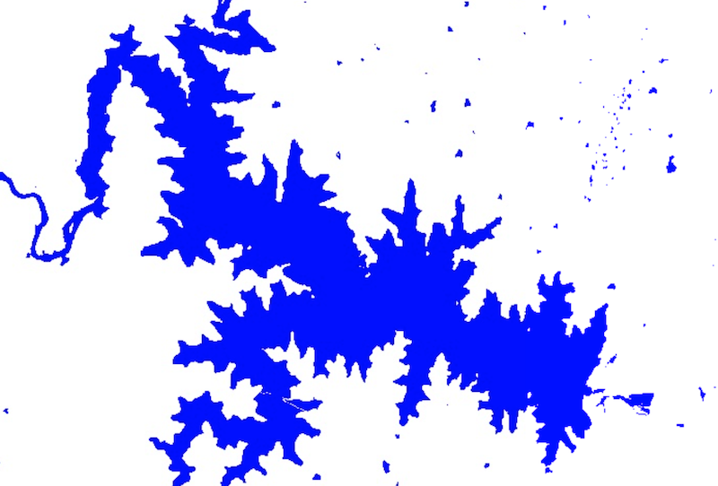
Detecting Surface Water with Dynamic World
// Example script showing how to extract water pixels
// from the Dynamic World dataset.

// Choose a region
var geometry = ee.Geometry.Polygon([[
  [76.37422, 12.5721],
  [76.37422, 12.3736],
  [76.62073, 12.3736],
  [76.62073, 12.5721]]
]);

// Choose a time period
// Some months may not have enough cloud-free observations
// Increase the time period if you have gaps in your results
var year = 2023;
var month = 1;
var startDate = ee.Date.fromYMD(year, month, 1);
var endDate = startDate.advance(1, 'month');

// Create and Visualize the Dynamic World probability composite
// for the chosen region and time period

// Filter the Dynamic World collection
var dwFiltered = ee.ImageCollection('GOOGLE/DYNAMICWORLD/V1')
  .filter(ee.Filter.date(startDate, endDate))
  .filter(ee.Filter.bounds(geometry));

// Select probability bands and compute mean probability during the period

var probabilityBands = [
  'water', 'trees', 'grass', 'flooded_vegetation', 'crops',
  'shrub_and_scrub', 'built', 'bare', 'snow_and_ice'
];

var probabilityImage = dwFiltered.select(probabilityBands).mean();

// Create and Visualize the Sentinel-2 composite
// for the chosen region and time period
var s2 = ee.ImageCollection('COPERNICUS/S2_HARMONIZED');

var filtered = s2.filter(ee.Filter.lt('CLOUDY_PIXEL_PERCENTAGE', 30))
  .filter(ee.Filter.date(startDate, endDate))
  .filter(ee.Filter.bounds(geometry));

var medianComposite = filtered.median();

var rgbVis = {
  min: 0.0,
  max: 3000,
  bands: ['B4', 'B3', 'B2'],
};

Map.centerObject(geometry);
Map.addLayer(medianComposite.clip(geometry), rgbVis, 'S2 Image');

// Visualize water probability
var probabilityVis = {
  min:0,
  max:1,
  bands: ['water'],
  palette: ['#f1eef6','#bdc9e1','#74a9cf','#2b8cbe','#045a8d']};

Map.addLayer(probabilityImage.clip(geometry), probabilityVis, 'Water Probability');


// **************************************************************
// 2. Extract Water
// **************************************************************

// Select a threshold for water probability
var waterThreshold = 0.5;

// Select all pixels where 'water' probability is > threshold
// The result is a binary image
var water = probabilityImage.select('water').gt(waterThreshold);

// [Optional] Include riparian vegetation around the banks
// var floodedVegetationThreshold = 0.3;
// var water = probabilityImage.select('water').gt(waterThreshold)
//   .or(probabilityImage.select('flooded_vegetation').gt(floodedVegetationThreshold));

// Visualize the water image
var waterVis = {min:0, max:1, palette: ['white', 'blue']};
Map.addLayer(water.clip(geometry), waterVis, 'Detected Water');
SAR
Sentinel-1 ARD Pre-Processing
This example script shows how to apply a Gamma MAP (Maximum A-posterior) Speckle Filter and Radiometric Terrain Correction to Sentinel-1 images using the Analysis Ready Data (ARD) preparation framework published by Mullissa, A. et. al.
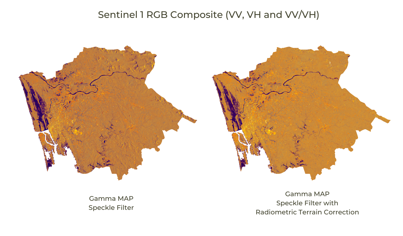
Gamma MAP Speckle filtering
// Example script that shows how to pre-process SAR data
// using Analysis Ready Data (ARD) Framework from
// https://github.com/adugnag/gee_s1_ard/tree/main

// Mullissa, A.; Vollrath, A.; Odongo-Braun, C.; Slagter, B.;
// Balling, J.; Gou, Y.; Gorelick, N.; Reiche, J.
// Sentinel-1 SAR Backscatter Analysis Ready Data Preparation
// in Google Earth Engine. Remote Sens. 2021, 13, 1954.
// https://doi.org/10.3390/rs13101954

// This script applies GAMMA MAP filter with border noise
// removal and radiometric terrain correction
var admin2 = ee.FeatureCollection("FAO/GAUL_SIMPLIFIED_500m/2015/level2");
var hydrosheds = ee.Image("WWF/HydroSHEDS/03VFDEM");

var startDate = '2018-08-10';
var endDate = '2018-08-23';

var selected = admin2.filter(ee.Filter.eq('ADM2_NAME', 'Ernakulam'));
var geometry = selected.geometry();
Map.centerObject(geometry);
Map.addLayer(geometry, {color: 'grey'}, 'Selected Admin-2');

// ************************************************************
// Sentinel-1 ARD Pre-Processing
// ************************************************************
var wrapper = require('users/adugnagirma/gee_s1_ard:wrapper');
var helper = require('users/adugnagirma/gee_s1_ard:utilities');

//-----------------------------------------------------------//
// DEFINE PARAMETERS
//-----------------------------------------------------------//

var parameters = {
  //1. Data Selection
  START_DATE: '2018-08-10',
  STOP_DATE: '2018-08-23',
  POLARIZATION:'VVVH',
  ORBIT : 'DESCENDING',
  GEOMETRY: geometry,

  //2. Additional Border noise correction
  APPLY_ADDITIONAL_BORDER_NOISE_CORRECTION: true,

  //3.Speckle filter
  APPLY_SPECKLE_FILTERING: true,
  SPECKLE_FILTER_FRAMEWORK: 'MULTI',
  SPECKLE_FILTER: 'GAMMA MAP',
  SPECKLE_FILTER_KERNEL_SIZE: 9,
  SPECKLE_FILTER_NR_OF_IMAGES: 10,

  //4. Radiometric terrain normalization
  APPLY_TERRAIN_FLATTENING: true,
  DEM: ee.Image('USGS/SRTMGL1_003'),
  TERRAIN_FLATTENING_MODEL: 'VOLUME',
  TERRAIN_FLATTENING_ADDITIONAL_LAYOVER_SHADOW_BUFFER: 0,

  //5. Output
  FORMAT : 'DB',
  CLIP_TO_ROI: true,
  SAVE_ASSETS: false
};

// Preprocess the S1 collection
var output = wrapper.s1_preproc(parameters);
var s1 = output[0];
var s1_preprocess = output[1];

// Function to add VV/VH ratio band
var addRatioBand = function(image) {
  var ratioBand = image.select('VV')
    .divide(image.select('VH')).rename('VV/VH');
  return image.addBands(ratioBand);
};

// Convert to DB and Add VV/VH ratio band
var speckleFiltered = s1_preprocess
  .map(helper.lin_to_db)
  .map(addRatioBand);

// Visualize
var sarComposite = speckleFiltered.mosaic().clip(geometry);

var visParams = {
  bands: ['VV', 'VH', 'VV/VH'],
  min:[-25, -25, 0],
  max:[0, 0, 2]
};
Map.addLayer(sarComposite, visParams, 'SAR RGB Visualization');
SAR Water Detection
// Script showing how to use Sentinel-1 data and
// static thresholding for water detection

var hydrobasins = ee.FeatureCollection("WWF/HydroSHEDS/v1/Basins/hybas_7");
var basin = hydrobasins.filter(ee.Filter.eq('HYBAS_ID', 4071139640));
var geometry = basin.geometry();
Map.addLayer(basin, {color: 'grey'}, 'Arkavathy Sub Basin');
Map.centerObject(geometry, 12);


// Use Sentinel-1 ARD Pre-Processing
// See https://github.com/adugnag/gee_s1_ard/
var wrapper = require('users/adugnagirma/gee_s1_ard:wrapper');
var helper = require('users/adugnagirma/gee_s1_ard:utilities');


var parameters = {
  // Input
  START_DATE: '2019-01-01',
  STOP_DATE: '2020-01-01',
  POLARIZATION:'VVVH',
  ORBIT : 'DESCENDING',
  GEOMETRY: geometry,

  // Speckle filter
  APPLY_SPECKLE_FILTERING: true,
  SPECKLE_FILTER_FRAMEWORK: 'MONO',
  SPECKLE_FILTER: 'REFINED LEE',

  // Output
  FORMAT : 'DB',
  CLIP_TO_ROI: true,
  SAVE_ASSETS: false
};

// Preprocess the S1 collection
var output = wrapper.s1_preproc(parameters);
var s1 = output[0];
var s1_preprocess = output[1];

// Convert to DB
var speckleFiltered = s1_preprocess
  .map(helper.lin_to_db);

// Mean is preferred for SAR data
var sarComposite = speckleFiltered.mean().select('VH');
var threshold = -25;
var sarWater = sarComposite.lt(threshold);
Map.addLayer(sarWater.clip(geometry).selfMask(),
  {min:0, max:1, palette: ['blue']}, 'Water');
Time Series Analysis
Mann Kendall Test
var taluks = ee.FeatureCollection("users/ujavalgandhi/gee-water-resources/kgis_taluks");
var chirps = ee.ImageCollection('UCSB-CHG/CHIRPS/PENTAD')


// We will compute the trend of total seasonal rainfall

// Introducting calendarRange()
var julyImages = chirps
  .filter(ee.Filter.calendarRange(7, 7, 'month'))
print(julyImages)

// Rainy season is June - September
var createSeasonalImage = function(year) {
  var startDate = ee.Date.fromYMD(year, 6, 1)
  var endDate = ee.Date.fromYMD(year, 9, 30)
  var seasonFiltered = chirps
    .filter(ee.Filter.date(startDate, endDate))
  // Calculate total precipitation
  var total = seasonFiltered.reduce(ee.Reducer.sum())
  return total.set({
    'system:time_start': startDate.millis(),
    'system:time_end': endDate.millis(),
    'year': year,
  })
}


// Aggregate Precipitation Data to get Annual Time-Series
var years = ee.List.sequence(1981, 2013)
var yearlyImages = years.map(createSeasonalImage)
print(yearlyImages)

var yearlyCol = ee.ImageCollection.fromImages(yearlyImages)


// Join the time series to itself
var afterFilter = ee.Filter.lessThan({
  leftField: 'system:time_start',
  rightField: 'system:time_start'
});

var joined = ee.ImageCollection(ee.Join.saveAll('after').apply({
  primary: yearlyCol,
  secondary: yearlyCol,
  condition: afterFilter
}));
print(joined)

// Mann-Kendall trend test
var sign = function(i, j) { // i and j are images
  return ee.Image(j).neq(i) // Zero case
      .multiply(ee.Image(j).subtract(i).clamp(-1, 1)).int();
};

var kendall = ee.ImageCollection(joined.map(function(current) {
  var afterCollection = ee.ImageCollection.fromImages(current.get('after'));
  return afterCollection.map(function(image) {
    // The unmask is to prevent accumulation of masked pixels that
    // result from the undefined case of when either current or image
    // is masked.  It won't affect the sum, since it's unmasked to zero.
    return ee.Image(sign(current, image)).unmask(0);
  });
  // Set parallelScale to avoid User memory limit exceeded.
}).flatten()).reduce('sum', 2);

var palette = ['red', 'white', 'green'];
// Stretch this as necessary.
Map.addLayer(kendall, {min:-30, max: 30, palette: palette}, 'kendall');
License
The course material (text, images, presentation, videos) is licensed under a Creative Commons Attribution 4.0 International License.
The code (scripts, Jupyter notebooks) is licensed under the MIT License. For a copy, see https://opensource.org/licenses/MIT
Kindly give appropriate credit to the original author as below:
Copyright © 2021 Ujaval Gandhi www.spatialthoughts.com
Citing and Referencing
You can cite the course materials as follows
- Gandhi, Ujaval, 2021. Google Earth Engine for Water Resources Management Course. Spatial Thoughts. https://courses.spatialthoughts.com/gee-water-resources-management.html
This course is offered as an instructor-led online class. Visit Spatial Thoughts to know details of upcoming sessions.
If you want to report any issues with this page, please comment below.