Google Earth Engine for Water Resources Management (Full Course)
Application-focused Introduction to Google Earth Engine.
Ujaval Gandhi
- Introduction
- Setting up the Environment
- Module 1: Google Earth Engine Fundamentals
- Module 2: Surface Water Mapping
- Module 3: Precipitation Time Series Analysis
- Module 4: Land Use Land Cover Classification
- Module 5: Flood Mapping
- Module 6: Drought Monitoring
- Module 7: Earth Engine Apps
- Supplement
- Data Credits
- License
- Citing and Referencing
![]()
Introduction
GIS and Remote Sensing plays a critical role in the management of water resources. Many practitioners in this field are constrained by the availability of tools and computing resources to use these techniques effectively. Recent advances in cloud computing technology have given rise to platforms such as Google Earth Engine, which provide free access to a large pool of computational resources and datasets. The course is designed for researchers in the water sector, academicians, water managers, and stakeholders with basic knowledge of Remote Sensing. It will enable them to leverage this platform for water resource management applications.
You will learn Google Earth Engine programming by building the following 5 complete applications:
- Surface Water Mapping
- Precipitation Time Series Analysis
- Land Use Land Cover Classification
- Flood Mapping
- Drought Monitoring
Note: Certification and Support are only available for participants in our paid instructor-led classes.

Setting up the Environment
Sign-up for Google Earth Engine
If you already have a Google Earth Engine account, you can skip this step.
Visit our GEE Sign-Up Guide for step-by-step instructions.
Get the Course Materials
The course material and exercises are in the form of Earth Engine scripts shared via a code repository.
- Click this link to open Google Earth Engine code editor and add the repository to your account.
- If successful, you will have a new repository named
users/ujavalgandhi/GEE-Water-Resources-Managementin the Scripts tab in the Reader section. - Verify that your code editor looks like below
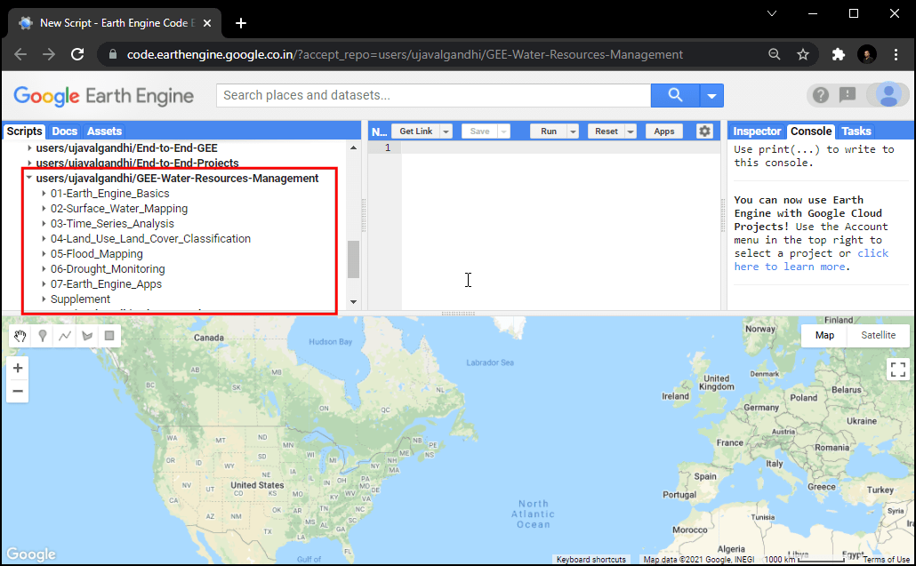
Code Editor After Adding the Class Repository
If you do not see the repository in the Reader section, click Refresh repository cache button in your Scripts tab and it will show up.
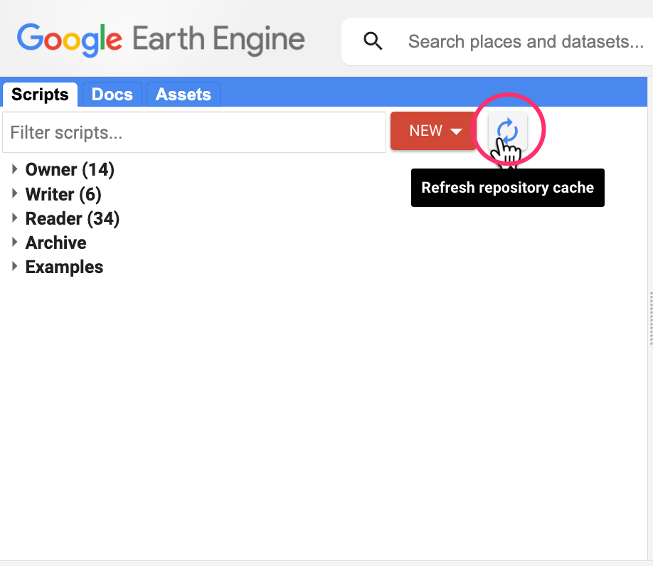
Refresh repository cache
Get the Course Videos
The course is accompanied by a set of videos covering the all the modules. These videos are recorded from our live instructor-led classes and are edited to make them easier to consume for self-study. We have 2 versions of the videos
YouTube
We have created a YouTube Playlist with separate videos for each script and exercise to enable effective online-learning. Access the YouTube Playlist ↗
Vimeo
We are also making combined full-length video for each module available on Vimeo. These videos can be downloaded for offline learning. Access the Vimeo Playlist ↗
Module 1: Google Earth Engine Fundamentals
In Module 1, you will gain the essential skills to find datasets, filter them to your region, clip them to your boundary, calculate remote sensing indices, extract water-bodies using thresholding techniques and export raster data.

01. Hello World
This script introduces the basic Javascript syntax and the video covers the programming concepts you need to learn when using Earth Engine. To learn more, visit Introduction to JavaScript for Earth Engine section of the Earth Engine User Guide.
The Code Editor is an Integrated Development Environment (IDE) for Earth Engine Javascript API. It offers an easy way to type, debug, run and manage code. Type the code below and click Run to execute it and see the output in the Console tab.
Tip: You can use the keyboard shortcut Ctrl+Enter to run the code in the Code Editor
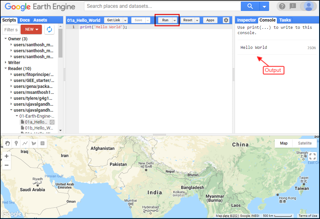
Hello World
print('Hello World');

// Variables
var city = 'Bengaluru';
var country = 'India';
print(city, country);

var population = 8400000;
print(population);

// List
var majorCities = ['Mumbai', 'Delhi', 'Chennai', 'Kolkata'];
print(majorCities);

// Dictionary
var cityData = {
  'city': city,
  'population': 8400000,
  'elevation': 930
};
print(cityData);

// Function
var greet = function(name) {
    return 'Hello ' + name;
};
print(greet('World'));

// This is a comment
Exercise
Saving Your Work
When you modify any script for the course repository, you may want to save a copy for yourself. If you try to click the Save button, you will get an error message like below
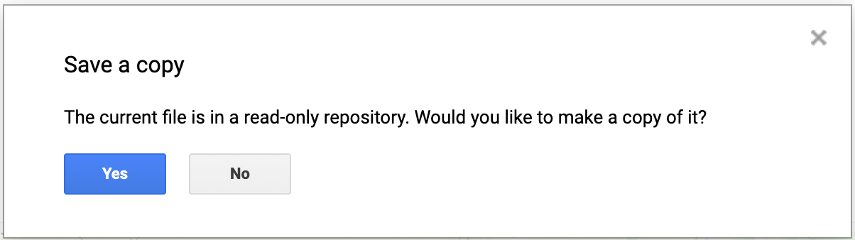
This is because the shared class repository is a Read-only repository. You can click Yes to save a copy in your repository. If this is the first time you are using Earth Engine, you will be prompted to choose a Earth Engine username. Choose the name carefully, as it cannot be changed once created.
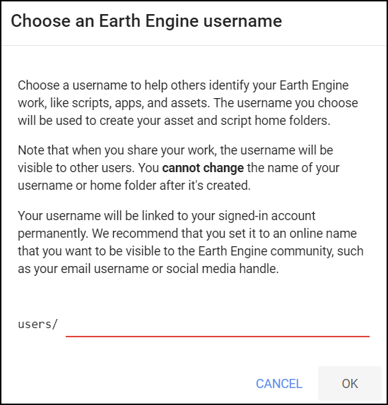
After entering your username, your home folder will be created. After that, you will be prompted to enter a new repository. A repository can help you organize and share code. Your account can have multiple repositories and each repository can have multiple scripts inside it. To get started, you can create a repository named default. Finally, you will be able to save the script.
02. Working with Image Collections
Most datasets in Earth Engine come as a ImageCollection.
An ImageCollection is a dataset that consists of images takes at
different time and locations - usually from the same satellite or data
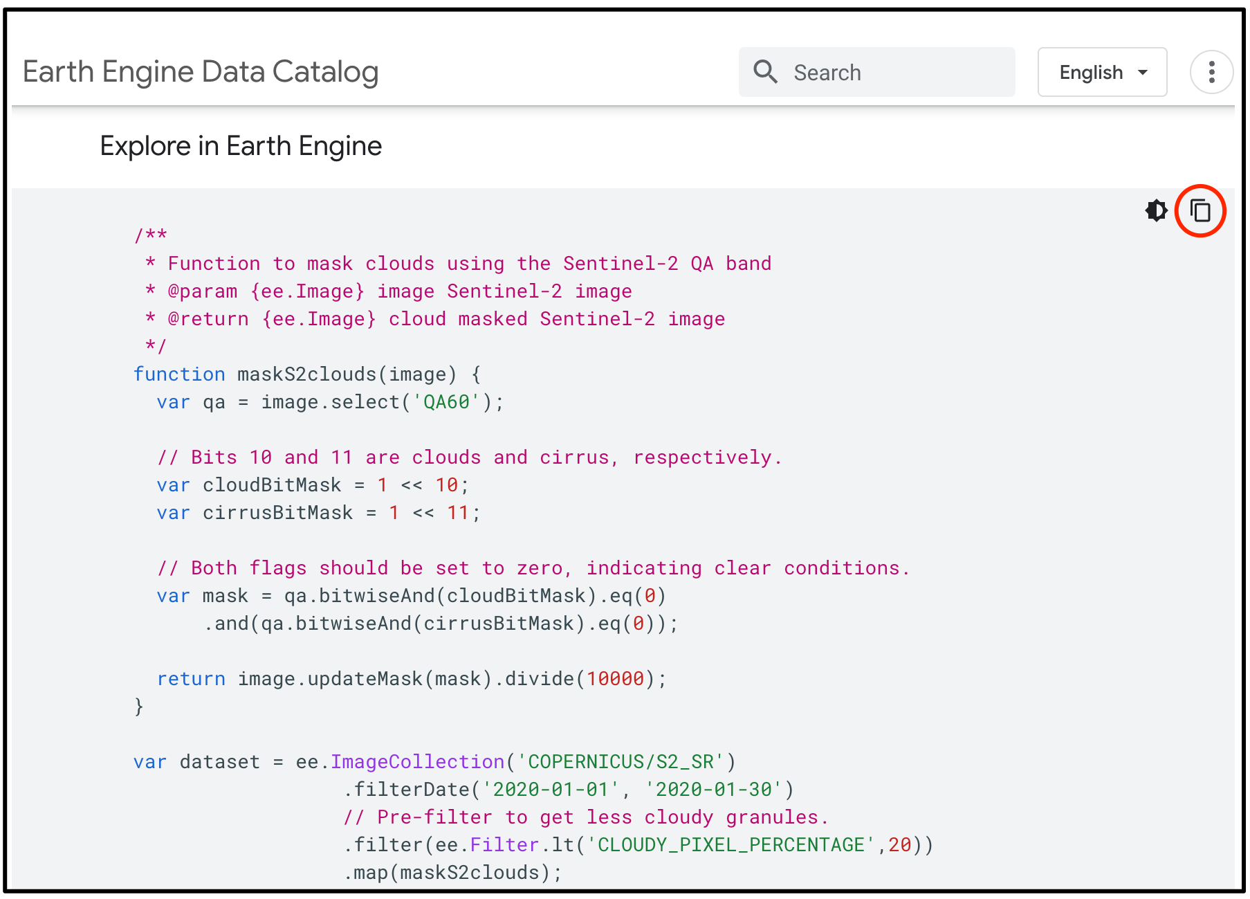
provider. You can load a collection by searching the Earth Engine
Data Catalog for the ImageCollection ID. Search for the
Sentinel-2 Level 2A dataset and you will find its id
COPERNICUS/S2_SR. Visit the Sentinel-2,
Level 2A page and see Explore in Earth Engine section to
find the code snippet to load and visualize the collection. This snippet
is a great starting point for your work with this dataset. Click the
Copy Code Sample button and paste the code into the
code editor. Click Run and you will see the image tiles load in
the map.
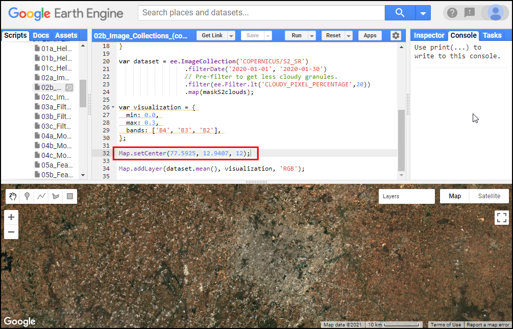
In the code snippet, You will see a function
Map.setCenter() which sets the viewport to a specific
location and zoom level. The function takes the X coordinate
(longitude), Y coordinate (latitude) and Zoom Level parameters ranging
from 1 (whole world) to 22 (pixel level). Replace the X and Y
coordinates with the coordinates of your city and click Run to
see the images of your city.
/**
 * Function to mask clouds using the Sentinel-2 QA band
 * @param {ee.Image} image Sentinel-2 image
 * @return {ee.Image} cloud masked Sentinel-2 image
 */
function maskS2clouds(image) {
  var qa = image.select('QA60');

  // Bits 10 and 11 are clouds and cirrus, respectively.
  var cloudBitMask = 1 << 10;
  var cirrusBitMask = 1 << 11;

  // Both flags should be set to zero, indicating clear conditions.
  var mask = qa.bitwiseAnd(cloudBitMask).eq(0)
      .and(qa.bitwiseAnd(cirrusBitMask).eq(0));

  return image.updateMask(mask).divide(10000);
}

// Map the function over one month of data and take the median.
// Load Sentinel-2 TOA reflectance data.
var dataset = ee.ImageCollection('COPERNICUS/S2_HARMONIZED')
                  .filterDate('2018-01-01', '2018-01-31')
                  // Pre-filter to get less cloudy granules.
                  .filter(ee.Filter.lt('CLOUDY_PIXEL_PERCENTAGE', 20))
                  .map(maskS2clouds);

var rgbVis = {
  min: 0.0,
  max: 0.3,
  bands: ['B4', 'B3', 'B2'],
};

Map.setCenter(77.61, 12.97, 10);
Map.addLayer(dataset.median(), rgbVis, 'RGB');
Exercise
/**
 * Function to mask clouds using the Sentinel-2 QA band
 * @param {ee.Image} image Sentinel-2 image
 * @return {ee.Image} cloud masked Sentinel-2 image
 */
function maskS2clouds(image) {
  var qa = image.select('QA60');

  // Bits 10 and 11 are clouds and cirrus, respectively.
  var cloudBitMask = 1 << 10;
  var cirrusBitMask = 1 << 11;

  // Both flags should be set to zero, indicating clear conditions.
  var mask = qa.bitwiseAnd(cloudBitMask).eq(0)
      .and(qa.bitwiseAnd(cirrusBitMask).eq(0));

  return image.updateMask(mask).divide(10000);
}

// Map the function over one month of data and take the median.
// Load Sentinel-2 TOA reflectance data.
var dataset = ee.ImageCollection('COPERNICUS/S2_HARMONIZED')
                  .filterDate('2018-01-01', '2018-01-31')
                  // Pre-filter to get less cloudy granules.
                  .filter(ee.Filter.lt('CLOUDY_PIXEL_PERCENTAGE', 20))
                  .map(maskS2clouds);

var rgbVis = {
  min: 0.0,
  max: 0.3,
  bands: ['B4', 'B3', 'B2'],
};

Map.setCenter(77.61, 12.97, 10);
Map.addLayer(dataset.median(), rgbVis, 'RGB');
03. Filtering Image Collections
The collection contains all imagery ever collected by the sensor. The
entire collections are not very useful. Most applications require a
subset of the images. We use filters to select the
appropriate images. There are many types of filter functions, look at
ee.Filter... module to see all available filters. Select a
filter and then run the filter() function with the filter
parameters.
We will learn about 3 main types of filtering techniques
- Filter by metadata: You can apply a filter on the
image metadata using filters such as
ee.Filter.eq(),ee.Filter.lt()etc. You can filter by PATH/ROW values, Orbit number, Cloud cover etc. - Filter by date: You can select images in a
particular date range using filters such as
ee.Filter.date(). - Filter by location: You can select the subset of
images with a bounding box, location or geometry using the
ee.Filter.bounds(). You can also use the drawing tools to draw a geometry for filtering.
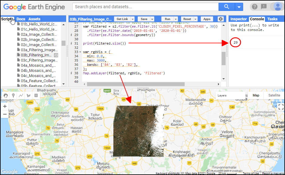
After applying the filters, you can use the .size()
function to check how many images match the filter criteria.
var geometry = ee.Geometry.Point([77.60412933051538, 12.952912912328241])
Map.centerObject(geometry, 10)

var s2 = ee.ImageCollection("COPERNICUS/S2_SR_HARMONIZED");

// Filter by metadata
var filtered = s2.filter(ee.Filter.lt('CLOUDY_PIXEL_PERCENTAGE', 30))

// Filter by date
var filtered = s2.filter(ee.Filter.date('2019-01-01', '2020-01-01'))

// Filter by location
var filtered = s2.filter(ee.Filter.bounds(geometry))

// Let's apply all the 3 filters together on the collection

// First apply metadata fileter
var filtered1 = s2.filter(ee.Filter.lt('CLOUDY_PIXEL_PERCENTAGE', 30))
// Apply date filter on the results
var filtered2 = filtered1.filter(
  ee.Filter.date('2019-01-01', '2020-01-01'))
// Lastly apply the location filter
var filtered3 = filtered2.filter(ee.Filter.bounds(geometry))

// Instead of applying filters one after the other, we can 'chain' them
// Use the . notation to apply all the filters together
var filtered = s2.filter(ee.Filter.lt('CLOUDY_PIXEL_PERCENTAGE', 30))
  .filter(ee.Filter.date('2019-01-01', '2020-01-01'))
  .filter(ee.Filter.bounds(geometry))

print(filtered.size());
Exercise
var geometry = ee.Geometry.Point([77.60412933051538, 12.952912912328241]);

var s2 = ee.ImageCollection("COPERNICUS/S2_SR_HARMONIZED");

var filtered = s2
  .filter(ee.Filter.lt('CLOUDY_PIXEL_PERCENTAGE', 30))
  .filter(ee.Filter.date('2019-01-01', '2020-01-01'))
  .filter(ee.Filter.bounds(geometry));

print(filtered.size());

// Exercise
// Delete the 'geometry' import
// Add a point at your chosen location
// Change the filter to find images from January 2023

// Note: If you are in a very cloudy region,
// make sure to adjust the CLOUDY_PIXEL_PERCENTAGE
04. Mosaics and Composites
The default order of the collection is by date. So when you display
the collection, it implicitly creates a mosaic with the latest pixels on
top. You can call .mosaic() on a ImageCollection to create
a mosaic image from the pixels at the top (i.e) first image in the
stack.
We can also create a composite image by applying selection criteria
to each pixel from all pixels in the stack. Here we use the
.median() function to create a composite where each pixel
value is the median of all pixels values at each pixel from the stack
for all matching bands.
Open in Code Editor ↗Tip: If you need to create a mosaic where the images are in a specific order, you can use the
.sort()function to sort your collection by a property first.
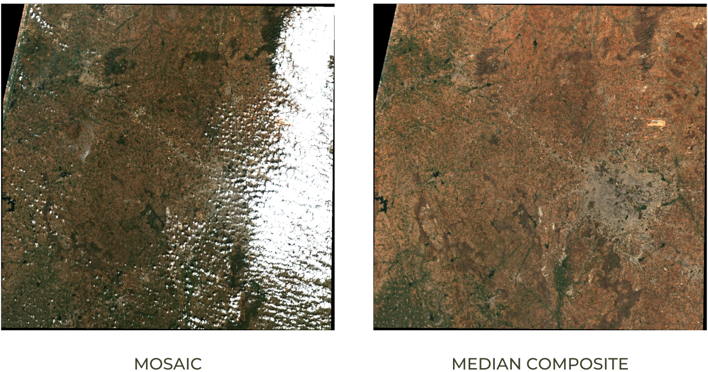
Mosaic vs. Median Composite
var geometry = ee.Geometry.Point([77.60412933051538, 12.952912912328241])
var s2 = ee.ImageCollection("COPERNICUS/S2_SR_HARMONIZED");

var rgbVis = {
  min: 0.0,
  max: 3000,
  bands: ['B4', 'B3', 'B2'],
};
var filtered = s2.filter(ee.Filter.lt('CLOUDY_PIXEL_PERCENTAGE', 30))
  .filter(ee.Filter.date('2019-01-01', '2020-01-01'))
  .filter(ee.Filter.bounds(geometry))

var mosaic = filtered.mosaic()

var medianComposite = filtered.median();

Map.centerObject(geometry, 10)
Map.addLayer(filtered, rgbVis, 'Filtered Collection');
Map.addLayer(mosaic, rgbVis, 'Mosaic');
Map.addLayer(medianComposite, rgbVis, 'Median Composite')
Exercise
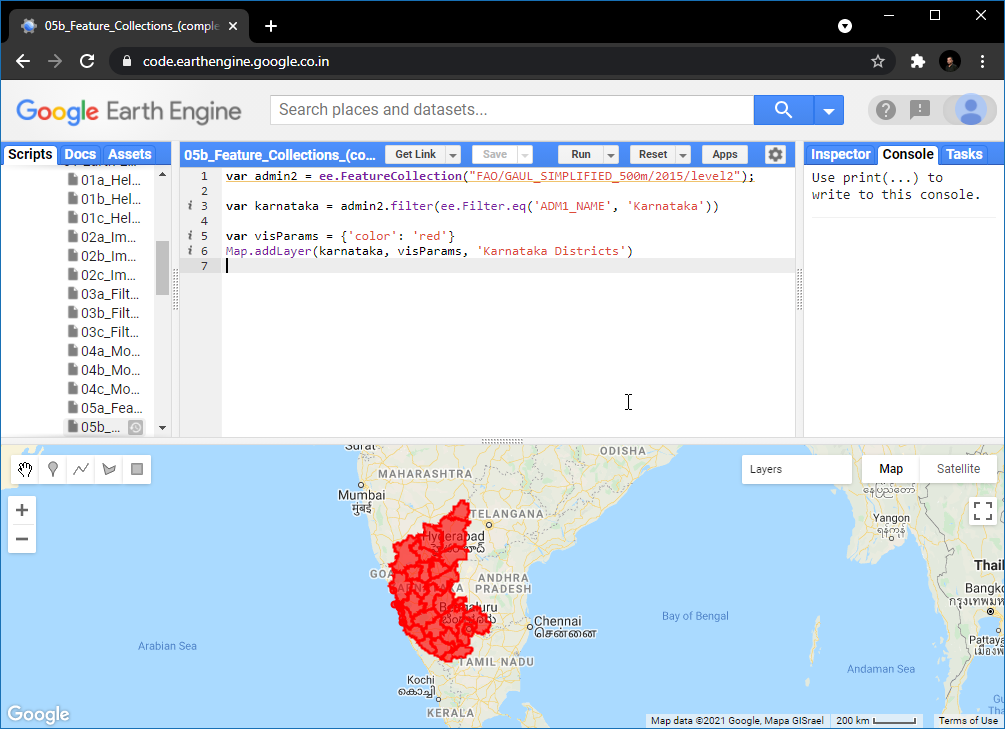
05. Feature Collections
Feature Collections are similar to Image Collections - but they contain Features, not images. They are equivalent to a Vector Layers in a GIS. We can load, filter and display Feature Collections using similar techniques that we have learned so far.
Search for GAUL Second Level Administrative Boundaries and
load the collection. This is a global collection that contains all
Admin2 boundaries. We can apply a filter using the
ADM1_NAME property to get all Admin2 boundaries
(i.e. Districts) from a state.
var admin2 = ee.FeatureCollection("FAO/GAUL_SIMPLIFIED_500m/2015/level2");

var filtered = admin2
  .filter(ee.Filter.eq('ADM1_NAME', 'Karnataka'))
  .filter(ee.Filter.eq('ADM2_NAME', 'Bangalore Urban'));

Map.centerObject(filtered);

Map.addLayer(filtered, {'color': 'red'}, 'Selected Admin2');
Exercise
06. Clipping
It is often desirable to clip the images to your area of interest.
You can use the clip() function to mask an image using
geometry.
While in Desktop softwares, clipping is used to remove the unnecessary portion of a large image to save computation time, but in the Earth Engine, clipping can increase the computation time. As described in the Earth Engine Coding Best Practices guide, avoid clipping or do it at the very end of your process.
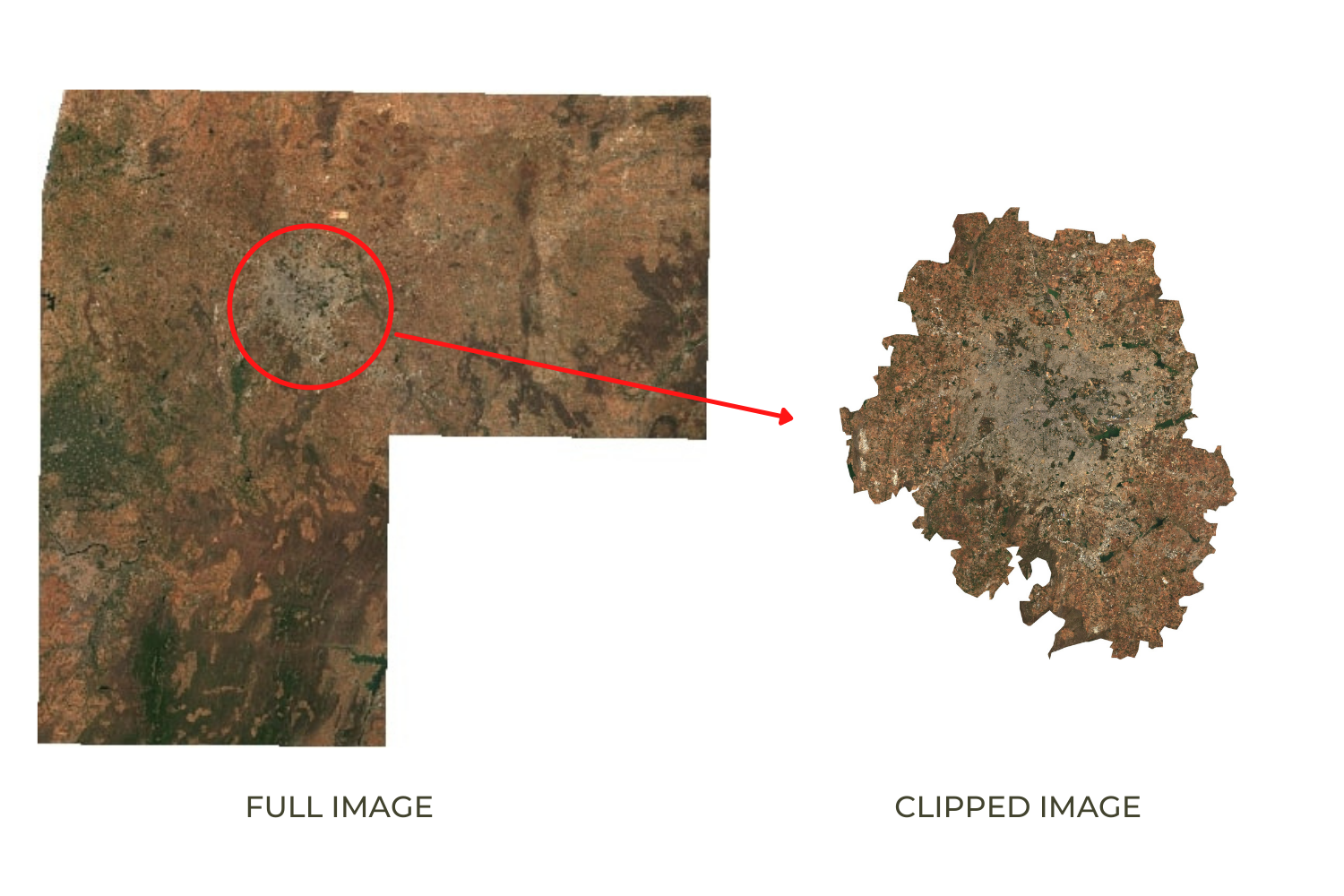
Full Image vs. Clipped Image
var admin2 = ee.FeatureCollection("FAO/GAUL_SIMPLIFIED_500m/2015/level2");
var s2 = ee.ImageCollection("COPERNICUS/S2_SR_HARMONIZED");

var filteredAdmin2 = admin2
  .filter(ee.Filter.eq('ADM1_NAME', 'Karnataka'))
  .filter(ee.Filter.eq('ADM2_NAME', 'Bangalore Urban'));

var geometry = filteredAdmin2.geometry();

var filteredS2 = s2.filter(ee.Filter.lt('CLOUDY_PIXEL_PERCENTAGE', 30))
  .filter(ee.Filter.date('2019-01-01', '2020-01-01'))
  .filter(ee.Filter.bounds(geometry));

var image = filteredS2.median();

var clipped = image.clip(geometry);

var rgbVis = {
  min: 0.0,
  max: 3000,
  bands: ['B4', 'B3', 'B2'],
};
Map.centerObject(geometry);
Map.addLayer(clipped, rgbVis, 'Clipped Composite');
Exercise
07. Calculating Indices
Spectral Indices are central to many aspects of remote sensing. For
almost all research/work, you will need to compute one spectral indices.
The most commonly used formula for calculating an index is computing the
Normalized Difference between 2 bands. Earth Engine provides a
helper function normalizedDifference() to help calculate
normalized indices, such as Normalized Difference Vegetation Index
(NDVI) or Modified Normalized Difference Water Index (MNDWI).
Some indices - such as the Automated Water Extraction Index (AWEI) -
require calculation using a more complex formula.In such cases, you can
use the expression() function which allow you to to
construct formula with common arithmetic operators. The script below
shows how to implement common water-related indices in Earth Engine.
Note that the AWEI formula expects the pixel values to be reflectances,
so we need to apply a scaling factor of 0.0001 to convert the Sentinel-2
band values to reflectances.
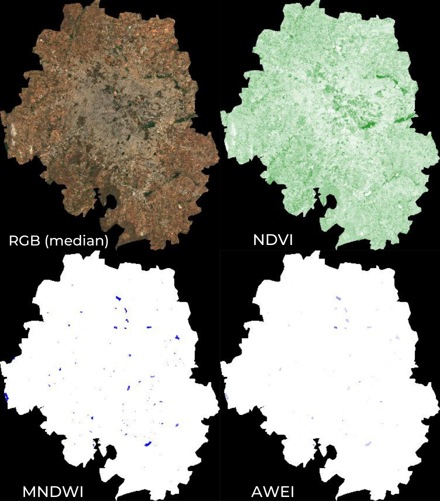
RGB, MNDWI, NDVI and AWEI images
var admin2 = ee.FeatureCollection("FAO/GAUL_SIMPLIFIED_500m/2015/level2");
var s2 = ee.ImageCollection("COPERNICUS/S2_SR_HARMONIZED");

var filteredAdmin2 = admin2
  .filter(ee.Filter.eq('ADM1_NAME', 'Karnataka'))
  .filter(ee.Filter.eq('ADM2_NAME', 'Bangalore Urban'));

var geometry = filteredAdmin2.geometry();

var filteredS2 = s2.filter(ee.Filter.lt('CLOUDY_PIXEL_PERCENTAGE', 30))
  .filter(ee.Filter.date('2019-01-01', '2020-01-01'))
  .filter(ee.Filter.bounds(geometry));

var image = filteredS2.median();

// Calculate  Normalized Difference Vegetation Index (NDVI)
// 'NIR' (B8) and 'RED' (B4)
var ndvi = image.normalizedDifference(['B8', 'B4']).rename(['ndvi']);

// Calculate Modified Normalized Difference Water Index (MNDWI)
// 'GREEN' (B3) and 'SWIR1' (B11)
var mndwi = image.normalizedDifference(['B3', 'B11']).rename(['mndwi']);

// Calculate Automated Water Extraction Index (AWEI)
// AWEI is a Multi-band Index that uses the following bands
// 'BLUE' (B2), GREEN' (B3), 'NIR' (B8), 'SWIR1' (B11) and 'SWIR2' (B12)

// Formula for AWEI is as follows
// AWEI = 4 * (GREEN - SWIR2) - (0.25 * NIR + 2.75 * SWIR1)

// For more complex indices, you can use the expression() function

// Note:
// For the AWEI formula, the pixel values need to converted to reflectances
// Multiplyng the pixel values by 'scale' gives us the reflectance value
// The scale value is 0.0001 for Sentinel-2 dataset

var awei = image.expression(
    '4*(GREEN - SWIR1) - (0.25*NIR + 2.75*SWIR2)', {
      'GREEN': image.select('B3').multiply(0.0001),
      'NIR': image.select('B8').multiply(0.0001),
      'SWIR1': image.select('B11').multiply(0.0001),
      'SWIR2': image.select('B12').multiply(0.0001),

}).rename('awei');


var rgbVis = {min: 0.0, max: 3000, bands: ['B4', 'B3', 'B2']};
var ndviVis = {min:0, max:1, palette: ['white', 'green']}
var ndwiVis = {min:0, max:0.5, palette: ['white', 'blue']}

Map.centerObject(geometry, 10)
Map.addLayer(image.clip(geometry), rgbVis, 'Image');
Map.addLayer(ndvi.clip(geometry), ndviVis, 'ndvi')
Map.addLayer(mndwi.clip(geometry), ndwiVis, 'mndwi')
Map.addLayer(awei.clip(geometry), ndwiVis, 'awei')
Exercise
There is another version of AWEI called AWEIsh. This index is useful where there are mountain or building shadows. This works best where there are shadows but no bright reflective surfaces (snow, roof). The expression for AWEI (sh) is as follows
AWEI (sh) = BLUE + 2.5*GREEN - 1.5*(NIR + SWIR1) - 0.25*SWIR2We have implemented both versions of AWEI in the script. Add them to the map and visualize both of them.
08. Computation on Images
Inspecting the MNDWI or AWEI index images, you will see that water
pixels have a higher value than other pixels. If we wanted to extract
those pixels, we can apply a threshold value to select all pixels above
a certain value. The result will be a binary image with pixel values 1
or 0. For all the pixels that matched the condition, the resulting value
will be 1, and for other pixels it will be 0. The conditions can be
written using the conditional operators like greater than
.gt(), lesser than .lt(), equal to
.eq(), greater than or equal to .gte(), etc.
We can also combine multiple layers to create a condition using the
boolean operators like AND .and(), OR
.or() functions. The script below shows how to implement
static thresholding in Earth Engine.
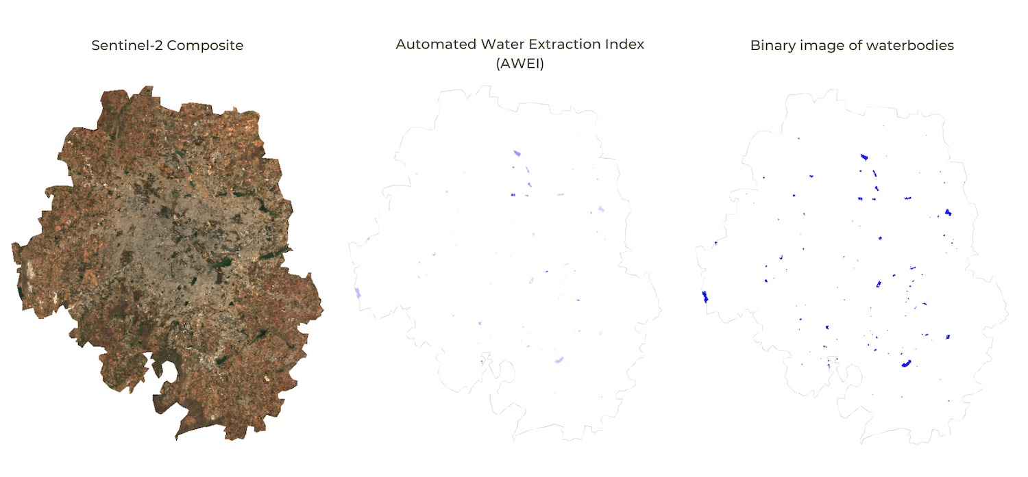
Extracting Waterbodies using a Simple Threshold
var admin2 = ee.FeatureCollection("FAO/GAUL_SIMPLIFIED_500m/2015/level2");
var s2 = ee.ImageCollection("COPERNICUS/S2_SR_HARMONIZED");

var filteredAdmin2 = admin2
  .filter(ee.Filter.eq('ADM1_NAME', 'Karnataka'))
  .filter(ee.Filter.eq('ADM2_NAME', 'Bangalore Urban'));

var geometry = filteredAdmin2.geometry();

var filteredS2 = s2.filter(ee.Filter.lt('CLOUDY_PIXEL_PERCENTAGE', 30))
  .filter(ee.Filter.date('2019-01-01', '2020-01-01'))
  .filter(ee.Filter.bounds(geometry));

var image = filteredS2.median();

var ndvi = image.normalizedDifference(['B8', 'B4']).rename(['ndvi']);
var mndwi = image.normalizedDifference(['B3', 'B11']).rename(['mndwi']);
var awei = image.expression(
    '4*(GREEN - SWIR1) - (0.25*NIR + 2.75*SWIR2)', {
      'GREEN': image.select('B3').multiply(0.0001),
      'NIR': image.select('B8').multiply(0.0001),
      'SWIR1': image.select('B11').multiply(0.0001),
      'SWIR2': image.select('B12').multiply(0.0001),
}).rename('awei');

// Simple Thresholding
var waterMndwi = mndwi.gt(0);
var waterAwei = awei.gt(0);

// Combining Multiple Conditions
var waterMultiple = ndvi.lt(0).and(mndwi.gt(0));

var rgbVis = {min: 0, max: 3000, bands: ['B4', 'B3', 'B2']};
var waterVis = {min:0, max:1, palette: ['white', 'blue']};

Map.centerObject(geometry, 10);
Map.addLayer(image.clip(geometry), rgbVis, 'Image');
Map.addLayer(waterMndwi.clip(geometry), waterVis, 'MNDWI - Simple threshold');
Map.addLayer(waterAwei.clip(geometry), waterVis, 'AWEI - Simple threshold');
Map.addLayer(waterMultiple.clip(geometry), waterVis, 'MNDWI and NDVI Threshold');
Exercise
Replace the selected region with the region of your choice and and adjust the MNDWI thresholds to extract the waterbodies.
Try different thresholds and add images to the map to compare
- Hint: Try negative thresholds -0.1 and -0.2
- Hint: Try positive thresholds 0.1 and 0.2
var admin2 = ee.FeatureCollection("FAO/GAUL_SIMPLIFIED_500m/2015/level2");
var s2 = ee.ImageCollection("COPERNICUS/S2_SR_HARMONIZED");

var filteredAdmin2 = admin2
  .filter(ee.Filter.eq('ADM1_NAME', 'Karnataka'))
  .filter(ee.Filter.eq('ADM2_NAME', 'Bangalore Urban'));

var geometry = filteredAdmin2.geometry();

var filteredS2 = s2.filter(ee.Filter.lt('CLOUDY_PIXEL_PERCENTAGE', 30))
  .filter(ee.Filter.date('2019-01-01', '2020-01-01'))
  .filter(ee.Filter.bounds(geometry));

var image = filteredS2.median();

var mndwi = image.normalizedDifference(['B3', 'B11']).rename(['mndwi']);

// Simple Thresholding
var waterMndwi = mndwi.gt(0);

// Excercise

// Replace the selected region with your choice
// And adjust the MNDWI thresholds to extract the waterbodies
// Try different thresholds and add images to the map to compare
// Hint: Try negative thresholds -0.1 and -0.2
// Hint: Try positive thresholds 0.1 and 0.2

var rgbVis = {min: 0, max: 3000, bands: ['B4', 'B3', 'B2']};
var waterVis = {min:0, max:1, palette: ['black', 'white']};

Map.centerObject(geometry, 10);
Map.addLayer(image.clip(geometry), rgbVis, 'Image');
Map.addLayer(waterMndwi.clip(geometry), waterVis, 'MNDWI (Threshold 0)');
09. Export
Earth Engine allows for exporting both vector and raster data to be
used in an external program. Vector data can be exported as a
CSV or a Shapefile, while Rasters can be
exported as GeoTIFF files. We will now export the
Sentinel-2 Composite as a GeoTIFF file.
During the export, we can export either a raw image or visualized image. The raw image will retain the original pixel values and is ideal if the image needs to be used for further analysis. The visualized image will generate an RGB visualization of the image. The visualized image will look exactly like you see it in Earth Engine with the visualization parameters, but original pixel values will be lost. The visualized image should not use it for analysis purposes.
Tip: Code Editor supports autocompletion of API functions using the combination Ctrl+Space. Type a few characters of a function and press Ctrl+Space to see autocomplete suggestions. You can also use the same key combination to fill all parameters of the function automatically.
var admin2 = ee.FeatureCollection("FAO/GAUL_SIMPLIFIED_500m/2015/level2");
var s2 = ee.ImageCollection("COPERNICUS/S2_SR_HARMONIZED");

var filteredAdmin2 = admin2
  .filter(ee.Filter.eq('ADM1_NAME', 'Karnataka'))
  .filter(ee.Filter.eq('ADM2_NAME', 'Bangalore Urban'));

var geometry = filteredAdmin2.geometry();

var filteredS2 = s2.filter(ee.Filter.lt('CLOUDY_PIXEL_PERCENTAGE', 30))
  .filter(ee.Filter.date('2019-01-01', '2020-01-01'))
  .filter(ee.Filter.bounds(geometry));

var image = filteredS2.median();

var ndvi = image.normalizedDifference(['B8', 'B4']).rename(['ndvi']);
var mndwi = image.normalizedDifference(['B3', 'B11']).rename(['mndwi']);

var waterMndwi = mndwi.gt(0);

var rgbVis = {min: 0, max: 3000, bands: ['B4', 'B3', 'B2']};
var waterVis = {min:0, max:1, palette: ['black', 'white']};

Map.centerObject(geometry, 10);

Map.addLayer(image.clip(geometry), rgbVis, 'Image');
Map.addLayer(waterMndwi.clip(geometry), waterVis, 'MNDWI');

var exportImage = image.select(['B4', 'B3', 'B2']);

Export.image.toDrive({
  image: exportImage.clip(geometry),
  description: 'Raw_Composite_Image',
  folder: 'earthengine',
  fileNamePrefix: 'composite',
  region: geometry,
  scale: 10,
  maxPixels: 1e10});

var visualizedImage = image.visualize(rgbVis);

Export.image.toDrive({
  image: visualizedImage.clip(geometry),
  description: 'Visualized_Composite_Image',
  folder: 'earthengine',
  fileNamePrefix: 'composite_visualized',
  region: geometry,
  scale: 10,
  maxPixels: 1e10
});
Once you run this script, the Tasks tab will be highlighted. Switch to the tab and you will see the tasks waiting. Click Run next to each task to start the process. On clicking the Run button, you will be prompted for a confirmation dialog. Verify the settings and click Run to start the export.
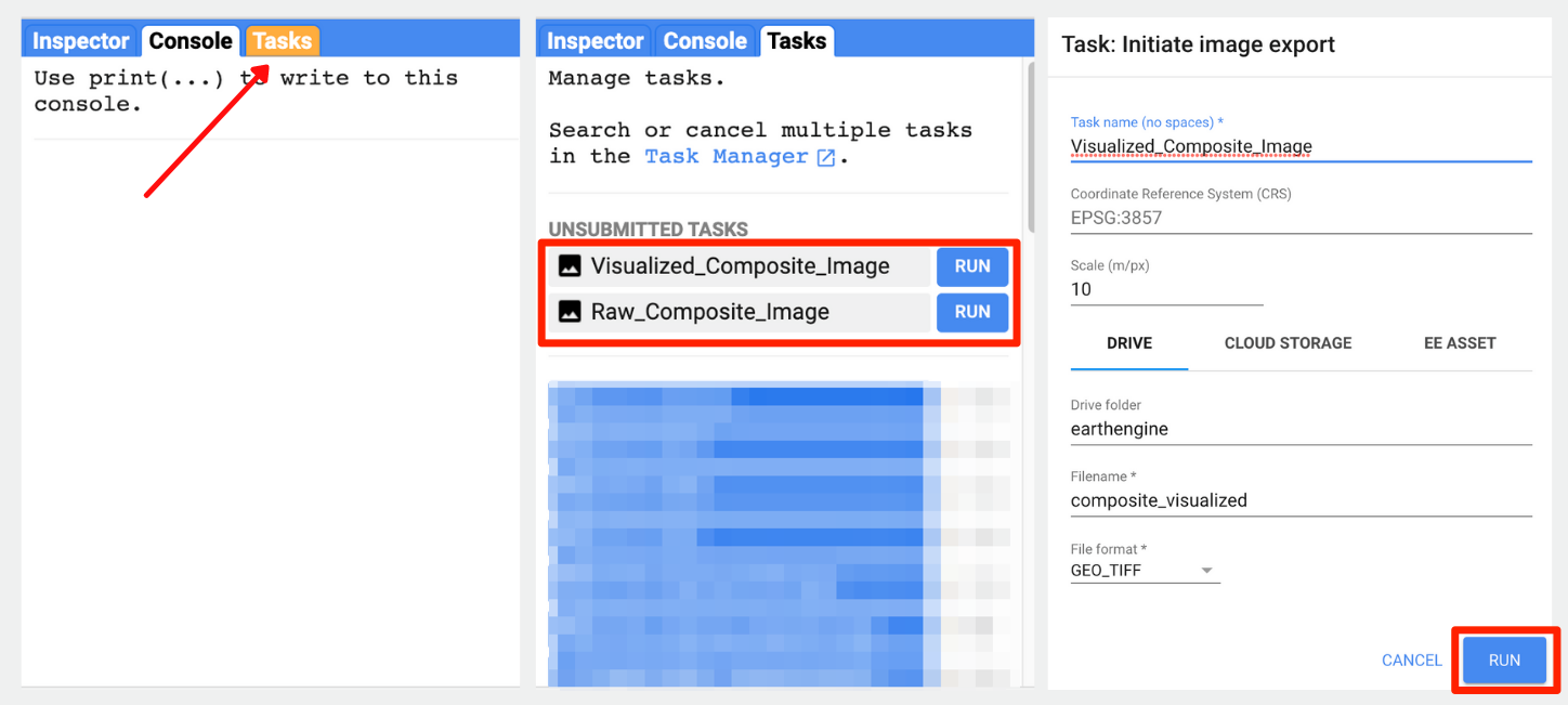
Console, Tasks and Confirmation.
Once the Export finishes, a GeoTiff file for each export task will be added to your Google Drive in the specified folder. You can download them and use it any program that reads GeoTiff files.
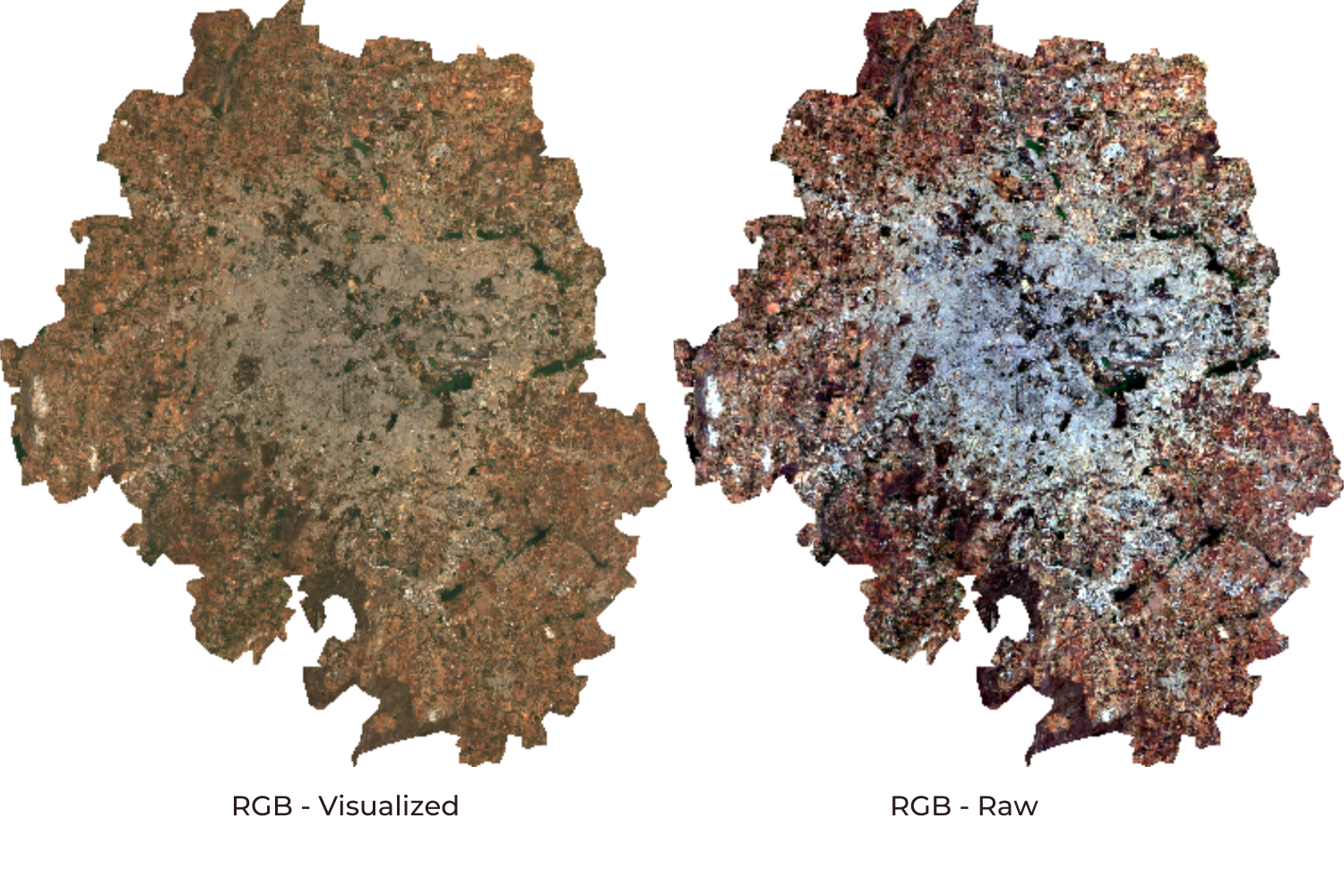
Visualized vs Raw
Module 2: Surface Water Mapping
In this Module, we will learn how to extract surface water polygons from a chosen watershed. We will be using in HydroSheds and JRC - Global Surface Water datasets. We will map the surface water for a chosen year, mask non-water pixels, apply morphological filters to remove fill holes and convert the raster image into polygons.

01. Load Global Surface Water Data
Lets load the JRC
Global Surface Water Mapping Layers. This data contains the
spatio-temporal distribution of surface water. It is a single image with
7 bands, where each band contains unique information. Let’s use the
occurrence band, which includes information on the
frequency of the water present from 1984-2020. The pixel value ranges
from 0-100, where 0 represents No trace of water in any year, and 100
represents water present in all 36 years.
Use the Inspector to find the frequency of water present in the location.
Open in Code Editor ↗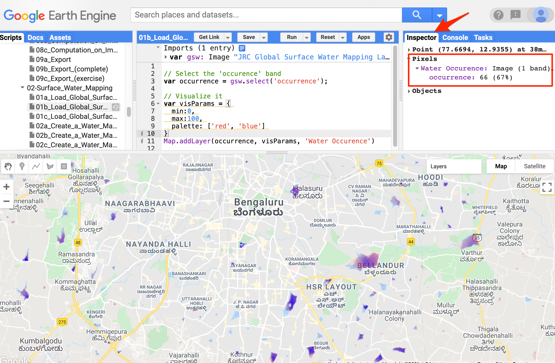
Frequency of water present over Bellandur lake
Exercise
The max_extent band gives information on whether a pixel
ever contained water or not, 0 represents the pixel has no water present
in any of the months, and 1 represents the pixel has contained water in
it for at least 1 month.
Load the max_extent band and visualize it with correct
parameters.
02. Create a Water Mask
Earth Engine has a mask function to represent the No
Data values in an Image. Any masked pixel of an image will not be
used for analysis or visualization. There are two types of masks
selfMask and updateMask.
The selfMask will remove all the pixel values with
zero. In the max_extent band visualization, we saw
the pixel value is either 0 or 1, the pixel value with 0 contains no
information, but the pixel value with 1 represents the water occurrence.
So to remove the No Data pixel within the image, we can use the selfMask
function. This will mask all pixel value with 0.
The updateMask will mask a primary image using
a mask image. A mask image is an image with 0 1 pixel value.
The primary image pixels overlaying with 0-pixel value in mask image
will be set as No Data and masked out.
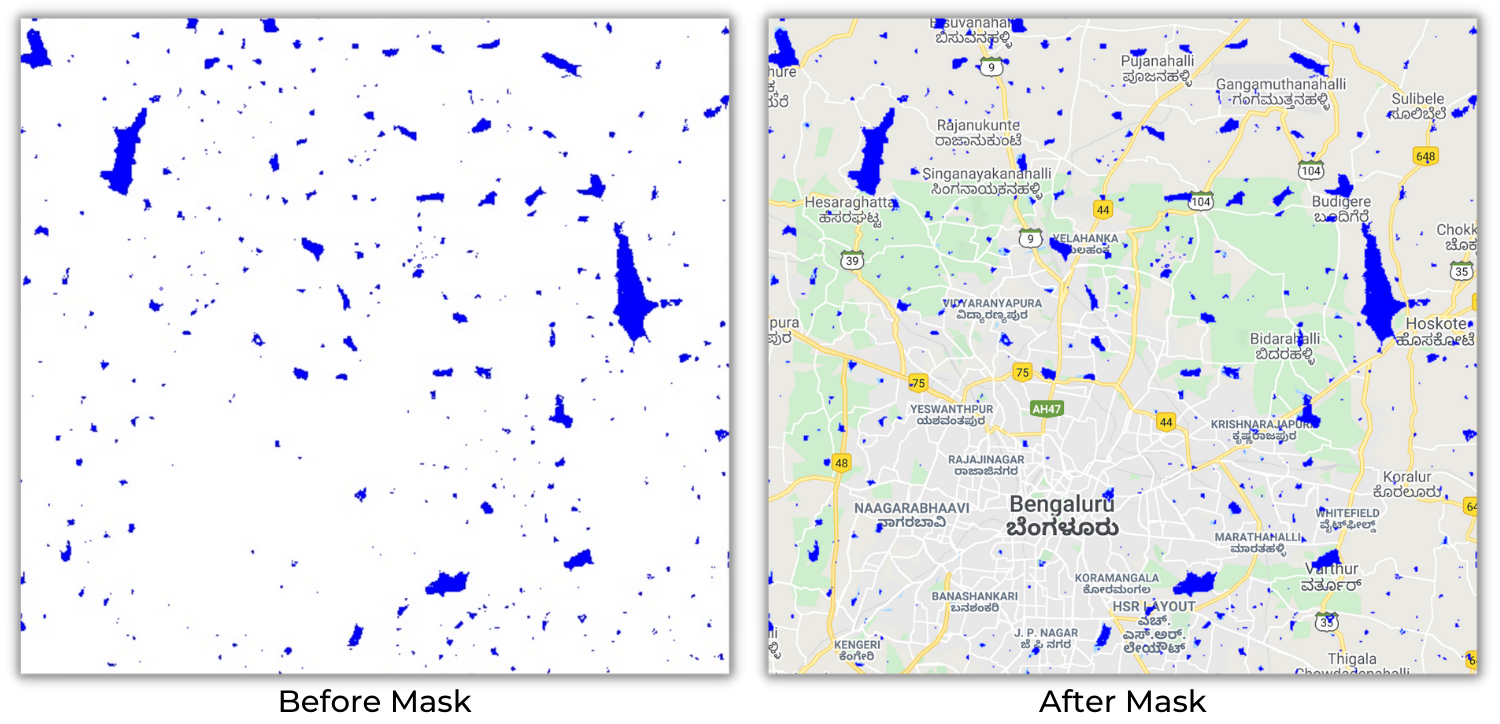
Before applying Mask vs After applying Mask
var gsw = ee.Image("JRC/GSW1_4/GlobalSurfaceWater");

// Select the 'max_extent' band
var water = gsw.select('max_extent');

// max_extent band has values 0 or 1
// We can remove the 0 values by masking the layer
// Mask needs to have 0 or 1 values
// 0 - remove the pixel
// 1 - keep the pixel

var masked = water.updateMask(water)

// There is a handy short-hand for masking out 0 values for a layer
// You can call selfMask() which will mask the image with itself
// Effectively removing 0 values and retaining non-zero values
var masked = water.selfMask()
Map.addLayer(masked, {}, 'Water');
Exercise
The seasonality band gives information on the number of
months water was present in a pixel. Pixel value ranges from 1 to 12, 1
represents water present for 1 month, and 12 represents water present
for 12 months in a year.
Select all pixels in which water present for more than 5 months in a year.
03. Find Lost Waterbodies
The transition band has water class changes between 1986
and 2020. It has 10
classes representing different changes, in which classes 3
and 6 represent permanent and seasonal water
loss. We can calculate the total area of surface water lost by
selecting both classes.
The binary operator eq is used to select a
particular class and create a binary image representing the availability
of the class. The boolean operator or is used to
create a binary image where either class value is present.
var gsw = ee.Image("JRC/GSW1_4/GlobalSurfaceWater");

// Select the 'transition' band
var water = gsw.select('transition');

var lostWater = water.eq(3).or(water.eq(6));

var visParams = {
  min:0,
  max:1,
  palette: ['white','red']
};

// Mask '0' value pixels
var lostWater = lostWater.selfMask();
Map.addLayer(lostWater, visParams, 'Lost Water');
Exercise
Use the transition band and find the total surface water
gain.
04. Get Yearly Water History
The JRC Yearly Water Classification History image collection contains the spatiotemporal map of surface water from 1984 to 2020. A total of 37 images represent 1 image for each year.
Let us filter this collection to visualize the surface water map of the year 2020. This data contains 4 bands, where bands 2 and 3 indicate water presence.
After filtering the Image Collection, the resultant would be a collection even if it contains just 1 image. We can use the function
.first()to extract the particular image.
var gswYearly = ee.ImageCollection("JRC/GSW1_4/YearlyHistory");

// Filter using the 'year' property

var filtered = gswYearly.filter(ee.Filter.eq('year', 2020));
var gsw2020 = ee.Image(filtered.first());

// Select permanent or seasonal water
var water2020 = gsw2020.eq(2).or(gsw2020.eq(3));

// Mask '0' value pixels
var water2020 = water2020.selfMask();

var visParams = {
  min:0,
  max:1,
  palette: ['white','blue']
};

Map.addLayer(water2020, visParams, '2020 Water');
Exercise
Use the JRC Yearly Water Classification History dataset
and visualize the surface water map for the year 2010.
05. Locate a SubBasin
The HydroSHEDS is a series
of data primarily developed by the World Wildlife Fund. It
contains a global level geo-reference stream network, watershed
boundaries, and drainage directions. We will use the
hydroBASINS, a feature collection containing drainage basin
boundaries. This data is created using SRTM DEM data. There are multiple
levels of hydroBASINS, ranging from 1 to 11. In level 1, the basin
boundaries are delineated as huge groups. Moving levels up, these
boundaries will be sub-divided into smaller boundaries.
We will use the Level 7 hydroBASINS feature collection to filter and locate a sun-basin called Arkavathy. The hydroBASINS doesn’t contain basin names, so basins should be visually located and filtered using the HYBAS_ID property to filter a particular basin boundary.
var hydrobasins = ee.FeatureCollection("WWF/HydroSHEDS/v1/Basins/hybas_7");

var basin = hydrobasins
  .filter(ee.Filter.eq('HYBAS_ID', 4071139640));

Map.centerObject(basin);
Map.addLayer(basin, {color: 'grey'}, 'Arkavathy Sub Basin');
Exercise
Using the Level 7 hydroBASINS, locate and filter a watershed basin in your region of interest.
06. Create a Surface Water Map
A raster image output can be post-processed using morphological operations to create a clean-looking surface map. There are different types of operations like Morphological Opening, Morphological Closing, and Majority Filtering.
Warning: We are processing the image here to clean it up to create a mapping product, but this changes the structure of the image and alters the statistics. Skip this step if your goal is to detect water pixels or compute the surface water area.
- The opening operation can reduce the salt and pepper noise in the image.
- The closing operation can fill holes and create a complete class.
- A majority filter will smooth the image. This operation should be used for mapping purposes only and not used while calculating statistics, as it will significantly alter the result.
Earth Engine has many functions to perform morphological operations
under ee.Image. Let’s use the Max_extent band
from Global Surface Water and fill holes to create a surface water map.
An Erosion operation follows a Dilation operation to
perform a closing operation, which translates as the focalMin
function chained with focalMax in the earth engine. Different
kernelType are available, let’s use the Square kernel
with 30 as search radius as the JRC’s Global Surface
Water spatial resolution is 30m. We can also define a custom kernel if
the required kernel is unavailable in kernelType.
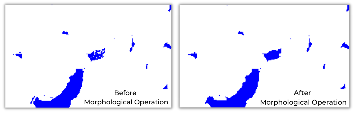
Before Operation vs After Operation
var gsw = ee.Image("JRC/GSW1_4/GlobalSurfaceWater");
var hydrobasins = ee.FeatureCollection("WWF/HydroSHEDS/v1/Basins/hybas_7");
var basin = hydrobasins
  .filter(ee.Filter.eq('HYBAS_ID', 4071139640))
var geometry = basin.geometry()
Map.centerObject(geometry, 10)

var water = gsw.select('max_extent');

var clipped = water.clip(geometry);

var visParams = {min:0, max:1, palette: ['white','blue']};
Map.addLayer(clipped, visParams, 'Surface Water') ;

// Do unmask() to replace masked pixels with 0
// This avoids extra pixels along the edges
var clipped = clipped.unmask(0);
// Perform a morphological closing to fill holes in waterbodies
var waterProcessed = clipped
  .focalMax({
    'radius':30,
    'units': 'meters',
    'kernelType': 'square'})
  .focalMin({
    'radius':30,
    'units': 'meters',
    'kernelType': 'square'});

Map.addLayer(waterProcessed, visParams, 'Surface Water (Processed)');
Exercise
By default, the total iteration is 1. We can increase it as required, so the kernel will pass through the image to perform the operation as many times as required.
Set the iteration parameter to 2 and execute the morphological closing operation.
var gsw = ee.Image("JRC/GSW1_4/GlobalSurfaceWater");
var hydrobasins = ee.FeatureCollection("WWF/HydroSHEDS/v1/Basins/hybas_7");
var basin = hydrobasins
  .filter(ee.Filter.eq('HYBAS_ID', 4071139640));
var geometry = basin.geometry();
Map.centerObject(geometry, 10);

var water = gsw.select('max_extent');

var clipped = water.clip(geometry);

var visParams = {min:0, max:1, palette: ['white','blue']};
Map.addLayer(clipped, visParams, 'Surface Water') ;

// Do unmask() to replace masked pixels with 0
// This avoids extra pixels along the edges
var clipped = clipped.unmask(0);
// Perform a morphological closing to fill holes in waterbodies
var waterProcessed = clipped
  .focalMax({
    'radius':30,
    'units': 'meters',
    'kernelType': 'square'})
  .focalMin({
    'radius':30,
    'units': 'meters',
    'kernelType': 'square'});
Map.addLayer(waterProcessed, visParams, 'Surface Water (Processed)');

// Exercise
// Replace the HYBAS_ID with the id of your selected basin
// Add an 'iterations' parameter with value 2 to
// focalMax and focalMin functions to further process the data
07. Convert Raster to Vector
After creating a final raster map, we can vectorize it. The
reduceToVectors function should be used with
countEvery reducer to convert a raster to a vector. This
reducer will connect all linked pixels of the same class into a single
feature and return a feature collection. By default, the connectedness
of a pixel is checked in cardinal directions only. To check the
connectedness of a pixel in the diagonal direction,
eightConnected should be set as true.
var gsw = ee.Image("JRC/GSW1_4/GlobalSurfaceWater");
var hydrobasins = ee.FeatureCollection("WWF/HydroSHEDS/v1/Basins/hybas_7");
var basin = hydrobasins
  .filter(ee.Filter.eq('HYBAS_ID', 4071139640));
var geometry = basin.geometry();
Map.centerObject(geometry, 10);

var water = gsw.select('max_extent');

var clipped = water.clip(geometry);

var visParams = {min:0, max:1, palette: ['white','blue']};
Map.addLayer(clipped, visParams, 'Surface Water', false) ;

// Do unmask() to replace masked pixels with 0
// This avoids extra pixels along the edges
var clipped = clipped.unmask(0);
// Perform a morphological closing to fill holes in waterbodies
var waterProcessed = clipped
  .focal_max({
    'radius':30,
    'units': 'meters',
    'kernelType': 'square'})
  .focal_min({
    'radius':30,
    'units': 'meters',
    'kernelType': 'square'});


var vector = waterProcessed.selfMask().reduceToVectors({
  reducer: ee.Reducer.countEvery(),
  geometry: geometry,
  scale: 30,
  maxPixels: 1e10,
  eightConnected: false
});
var visParams = {color: 'blue'};
Map.addLayer(vector, visParams, 'Surface Water Polygons');
Exercise
The final feature collection will contain the class value from the pixel as the label property. Since the raster is a binary image with 0 - 1 value, the label with value 1 will represent the water bodies.
Use the eq filter and filter the water bodies alone.
var gsw = ee.Image("JRC/GSW1_4/GlobalSurfaceWater");
var hydrobasins = ee.FeatureCollection("WWF/HydroSHEDS/v1/Basins/hybas_7");
var basin = hydrobasins.filter(ee.Filter.eq('HYBAS_ID', 4071139640))
var geometry = basin.geometry()
Map.centerObject(geometry, 10)

var water = gsw.select('max_extent');

var clipped = water.clip(geometry)

var visParams = {min:0, max:1, palette: ['white','blue']}
Map.addLayer(clipped, visParams, 'Surface Water', false)

// Do unmask() to replace masked pixels with 0
// This avoids extra pixels along the edges
var clipped = clipped.unmask(0);
// Perform a morphological closing to fill holes in waterbodies
var waterProcessed = clipped
  .focal_max({
    'radius':30,
    'units': 'meters',
    'kernelType': 'square'})
  .focal_min({
    'radius':30,
    'units': 'meters',
    'kernelType': 'square'});


var vector = waterProcessed.selfMask().reduceToVectors({
  reducer: ee.Reducer.countEvery(),
  geometry: geometry,
  scale: 30,
  maxPixels: 1e10,
  eightConnected: false
});

Map.addLayer(vector, {color: 'cyan'}, 'All Surface Water Polygons');

// Exercise
// 'vector' is a FeatureCollection of water polygons
// The following block adds a property 'area'
// to each polygon with its area in sq.meters.
var vectorArea = vector.map(function(x){
  var a = ee.Feature(x).area({maxError: 1});
  return x.set({'area':a});
});

// Apply a filter on the 'vectorArea' FeatureCollection
// to select water polygons larger than 1 Acre
// 1 Acre = 4046.86 sq. meters.

// Display the results on the map
Module 3: Precipitation Time Series Analysis
The main advantage of the gridded precipitation datasets is that they offer a consistent long-term time-series. We will cover the basics of gridded rainfall datasets, how to aggregate them to the requirement temporal resolution, prepare a time-series and perform pixel-wise trend analysis.
But to fully leverage the computation power of Earth Engine for our analysis, we must first learn about techniques for writing efficient parallel computing code. The Earth Engine API uses Map/Reduce paradigm for parallel computing.

01. Mapping a Function
This script introduces the basics of the Earth Engine API. Here we map a list of objects over a function to perform a task on all the objects. While defining a function, it should return a result after computation, which can be stored in a variable. To learn more, visit the Earth Engine Objects and Methods section of the Earth Engine User Guide.
Apart from other regular strings and numbers, the earth engine can
understand dates. Under ee.Date there are many functions by
which dates can be defined or converted from one format to another.
// Let's see how to take a list of numbers and add 1 to each element
var myList = ee.List.sequence(1, 10);

// Define a function that takes a number and adds 1 to it
var myFunction = function(number) {
  return number + 1;
};
print(myFunction(1));

//Re-Define a function using Earth Engine API
var myFunction = function(number) {
  return ee.Number(number).add(1);
};

// Map the function of the list
var newList = myList.map(myFunction);
print(newList);

// Let's write another function to square a number
var squareNumber = function(number) {
  return ee.Number(number).pow(2);
};
var squares = myList.map(squareNumber);
print(squares);

// Extracting value from a list

var value = newList.get(0);
print(value);

// Casting

// Let's try to do some computation on the extracted value
//var newValue = value.add(1)
//print(newValue)

// You get an error because Earth Engine doesn't know what is the type of 'value'
// We need to cast it to appropriate type first
var value = ee.Number(value);
var newValue = value.add(1);
print(newValue);

// Dates
// For any date computation, you should use ee.Date module

var date = ee.Date.fromYMD(2019, 1, 1);
var futureDate = date.advance(1, 'year');
print(futureDate);
Exercise
Define the function createDate, map the
weeks list as input. The function should return dates
incremented by the week number.
02. Reducers
A Reduce operation allows you to compute statistics on a
large amount of inputs. In Earth Engine, you need to run reduction
operation when creating composites, calculating statistics, doing
regression analysis etc. The Earth Engine API comes with a large number
of built-in reducer functions (such as ee.Reducer.sum(),
ee.Reducer.histogram(), ee.Reducer.linearFit()
etc.) that can perform a variety of statistical operations on input
data. You can run reducers using the reduce() function.
Earth Engine supports running reducers on all data structures that can
hold multiple values, such as Images (reducers run on different bands),
ImageCollection, FeatureCollection, List, Dictionary etc. The script
below introduces basic concepts related to reducers.
// Computing stats on a list
var myList = ee.List.sequence(1, 10);
print(myList);

// Use a reducer to compute min and max in the list
var mean = myList.reduce(ee.Reducer.mean());
print(mean);

var geometry = ee.Geometry.Polygon([[
  [82.60642647743225, 27.16350437805251],
  [82.60984897613525, 27.1618529901377],
  [82.61088967323303, 27.163695288375266],
  [82.60757446289062, 27.16517483230927]
]]);
var s2 = ee.ImageCollection("COPERNICUS/S2_HARMONIZED");
Map.centerObject(geometry);

// Apply a reducer on a image collection
var filtered = s2.filter(ee.Filter.lt('CLOUDY_PIXEL_PERCENTAGE', 30))
  .filter(ee.Filter.date('2019-01-01', '2020-01-01'))
  .filter(ee.Filter.bounds(geometry))
  .select('B.*');

print(filtered.size());
var collMean = filtered.reduce(ee.Reducer.mean());
print('Reducer on Collection', collMean);

var image = ee.Image('COPERNICUS/S2_HARMONIZED/20190223T050811_20190223T051829_T44RPR');
var rgbVis = {min: 0.0, max: 3000, bands: ['B4', 'B3', 'B2']};
Map.addLayer(image, rgbVis, 'Image');
Map.addLayer(geometry, {color: 'red'}, 'Farm');
// If we want to compute the average value in each band,
// we can use reduceRegion instead
var stats = image.reduceRegion({
  reducer: ee.Reducer.mean(),
  geometry: geometry,
  scale: 100,
  maxPixels: 1e10
  });
print(stats);

// Result of reduceRegion is a dictionary.
// We can extract the values using .get() function
print('Average value in B4', stats.get('B4'));
Exercise
// Below is a list of pixel values in an image
var pixelValues = ee.List(
  [1200, 2800, 1800, 1300, 3400, 2100, 1600]
);

// Exercise
// a. Divide each number by 10000 to get reflectances.
//    Hint: map() a function on the list
// b. Calculate the mean and standard deviation of computed reflectances.
//    Hint: reduce() the results
03. Calculating Total Rainfall
The CHIRPS Pentad is 5 days composite of rainfall at ~6 km spatial resolution. To compute this data, both satellite and grounds values are considered. To read more about the methodology, visit nature.com
Using this image collection, lets filter all the images for 2017. To
get a yearly rainfall we can reduce the collection using
reduce function with sum reducer. This will return
a single global image where each pixel represent the total annual
rainfall value in mm at that location. Now to get a annual
average rainfall at a particular region of interest, we can do a
reduceRegions with a mean reducer over the region.
This reducer will reduce the region’s image and return a dictionary. The
dictionary will contain the average value of all the bands in the image,
which can be extracted using the get function.
var geometry = ee.Geometry.Polygon([[
  [77.43833, 13.0497],
  [77.43833, 12.8141],
  [77.72123, 12.8141],
  [77.72123, 13.0497]
]]);

Map.addLayer(geometry, {}, 'ROI');

var chirps = ee.ImageCollection("UCSB-CHG/CHIRPS/PENTAD");

var startDate = ee.Date.fromYMD(2017, 1,1);
var endDate = startDate.advance(1, 'year');
var filtered = chirps
  .filter(ee.Filter.date(startDate, endDate));

// Calculate yearly rainfall
var total = filtered.reduce(ee.Reducer.sum());

var palette = ['#ffffcc','#a1dab4','#41b6c4','#2c7fb8','#253494'];
var visParams = {
  min:0,
  max: 2000,
  palette: palette
};
Map.addLayer(total, visParams, 'Total Precipitation');

Map.centerObject(geometry, 10);

// Calculate average rainfall across a region
var stats = total.reduceRegion({
  reducer: ee.Reducer.mean(),
  geometry: geometry,
  scale: 5566,
});

print(stats);

print('Average rainfall across ROI :', stats.getNumber('precipitation_sum'));
Output
Average rainfall across ROI :
1345.867775034789
Exercise
Update the date rage for monsoon season(1 June - 30 September) in India.
04. Aggregating Time Series
In the previous exercise, we aggregated to get the average rainfall across a region. Let’s compute a time series representing the total rainfall of each month in 2019.
Earth Engine has a function called ee.Date.fromYMD to
create a date from Year, Month, and Date.
Using this function and .advance(), we can create the
filter date to filter the image collection to a particular month. Then
with reduce function with sum as reducer, the
monthly image collection is aggregated to the monthly total image. This
newly created image won’t have any properties. Hence using the
.set() function, we have to assign the Year,
Month, system:time_start, and system:time_end
properties. With the above procedure in the sequence, we can create a
function to input the month’s number and return the monthly total
precipitation image.
We can create the month’s list using ee.List.sequence
and map it to the function built. Since the mapped object is of type
List, the resultant will also be a list with 12 images. This list of
images can be converted back as Image Collection using
ee.ImageCollection.fromYMD. Once we have the collection
print, it will contain 12 images representing the month’s total
precipitation.
The system:time_start is a unique property that the earth engine can natively understand. It is the Unix Timestamp that is used to create a time series chart.
var chirps = ee.ImageCollection("UCSB-CHG/CHIRPS/PENTAD");


var year = 2019;
var startDate = ee.Date.fromYMD(year, 1, 1);
var endDate = startDate.advance(1, 'year');
var yearFiltered = chirps
  .filter(ee.Filter.date(startDate, endDate));
// CHIRPS collection has 1 image for every pentad (5-days)
// The collection is filtered for 1 year and the time-series
// now has 72 images
print(yearFiltered);

// We need to aggregate this time series to compute
// monthly images

// Create a list of months
var months = ee.List.sequence(1, 12);

// Write a function that takes a month number
// and returns a monthly image
var createMonthlyImage = function(month) {
  var startDate = ee.Date.fromYMD(year, month, 1);
  var endDate = startDate.advance(1, 'month');
  var monthFiltered = yearFiltered
    .filter(ee.Filter.date(startDate, endDate));
  // Calculate total precipitation
  var total = monthFiltered.reduce(ee.Reducer.sum());
  return total.set({
    'system:time_start': startDate.millis(),
    'system:time_end': endDate.millis(),
    'year': year,
    'month': month});
};

// map() the function on the list  of months
// This creates a list with images for each month in the list
var monthlyImages = months.map(createMonthlyImage);
// Create an imagecollection
var monthlyCollection = ee.ImageCollection.fromImages(monthlyImages);
print('Monthly Collection', monthlyCollection);
Exercise
Filter the monthlyCollection for the months June, July,
August and September.
05. Charting Monthly Rainfall
Now we can put together all the skills we have learned so far -
filter, map, and reduce to create a chart of monthly total rainfall in
the year 2019 over a region. Earth Engine API supports charting
functions based on the Google Chart API. There are various charts to
use, from which we use the ui.Chart.image.series() function
to create a time-series chart.
Image series chart accepts an image collection,
geometry, scale, and reducer. The geometry in
the region of interest, reducer in the reduction operation the region of
interest should be aggregated if the geometry is a polygon. Scale is the
resolution at which the image should be reduced. Using
.setOptions, we can customize the chart to our needs.
Charting itself is vast, and all function are self explanatory. Google Earth Engine documentation provides all types of charting examples
var geometry = ee.Geometry.Point([77.58253382230242, 12.942038375108362]);
Map.addLayer(geometry, {}, 'POI')

var chirps = ee.ImageCollection("UCSB-CHG/CHIRPS/PENTAD")

var year = 2019
var startDate = ee.Date.fromYMD(year, 1, 1)
var endDate = startDate.advance(1, 'year')
var yearFiltered = chirps
  .filter(ee.Filter.date(startDate, endDate))
// CHIRPS collection has 1 image for every pentad (5-days)
// The collection is filtered for 1 year and the time-series
// now has 72 images
print(yearFiltered)

// We need to aggregate this time series to compute
// monthly images

// Create a list of months
var months = ee.List.sequence(1, 12)

// Write a function that takes a month number
// and returns a monthly image
var createMonthlyImage = function(month) {
  var startDate = ee.Date.fromYMD(year, month, 1);
  var endDate = startDate.advance(1, 'month');
  var monthFiltered = yearFiltered
    .filter(ee.Filter.date(startDate, endDate));
  // Calculate total precipitation
  var total = monthFiltered.reduce(ee.Reducer.sum());
  return total.set({
    'system:time_start': startDate.millis(),
    'system:time_end': endDate.millis(),
    'year': year,
    'month': month});
};

// map() the function on the list  of months
// This creates a list with images for each month in the list
var monthlyImages = months.map(createMonthlyImage);
// Create an imagecollection
var monthlyCollection = ee.ImageCollection.fromImages(monthlyImages);
print(monthlyCollection);

// Create a chart of monthly rainfall for a location
var chart = ui.Chart.image.series({
  imageCollection: monthlyCollection,
  region: geometry,
  reducer: ee.Reducer.mean(),
  scale: 5566
}).setOptions({
      lineWidth: 1,
      pointSize: 3,
      title: 'Monthly Rainfall at Bengaluru',
      vAxis: {title: 'Rainfall (mm)'},
      hAxis: {title: 'Month', gridlines: {count: 12}}
});
print(chart);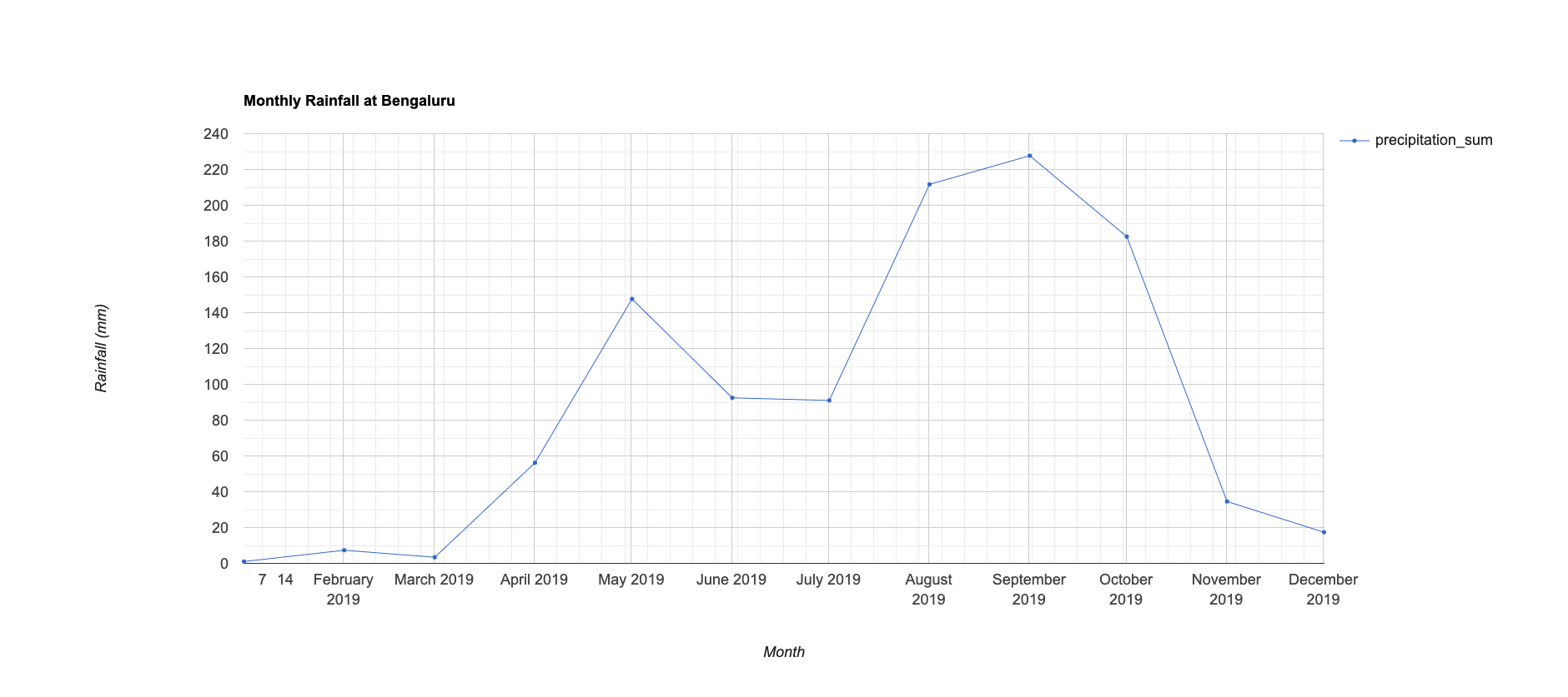
2019 - Monthly rainfall
Exercise
Change the geometry to your location, compute the monthly total rainfall. Download the timeseries chart generated.
06. Import
You can import vector or raster data into Earth Engine. We will now
import a shapefile of Taluk for a state
in India. Unzip the Taluk.rar into a folder on your
computer. In the Code Editor, go to Assets → New → Table Upload →
Shape Files. Select the .cpj, .sbn,
.shp, .shx, .dbfand
.prj files. Enter Taluk_Boundary as the
Asset Name and click Upload. In the Tasks tab
you can see the progress of the upload. Once the ingestion is complete
you will have a new asset in the Assets tab. The shapefile will
be imported as a Feature Collection in Earth Engine. Select the
Taluk_Boundary asset and click Import. You can
then visualize the imported data.
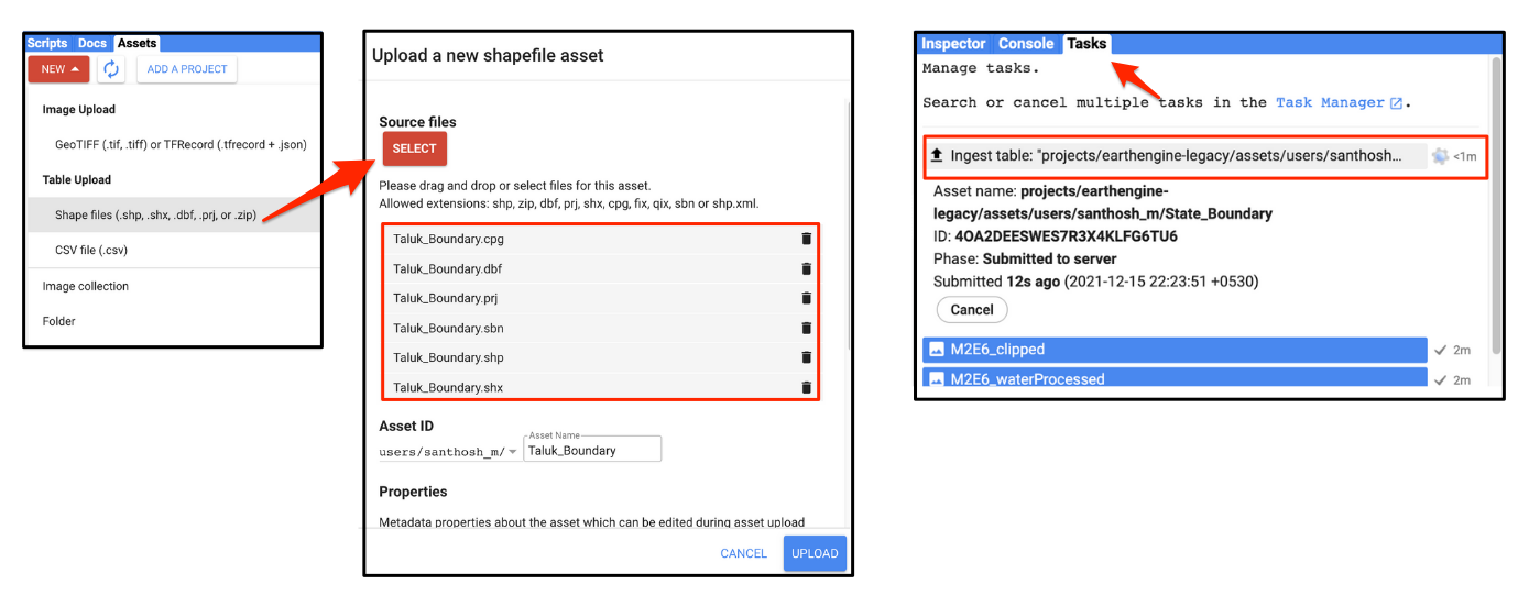
Importing a Shapefile
// Import the collection
var taluks = ee.FeatureCollection("users/ujavalgandhi/gee-water-resources/kgis_taluks");

// Visualize the collection
Map.centerObject(taluks)
Map.addLayer(taluks, {color: 'gray'}, 'Taluks')

// Function to add a new property 'area_sqkm'
// Function takes a feature and returns the feature
// with a new property
var addArea = function(f) {
  var area = ee.Number(f.get('SHAPE_STAr')).divide(1e6)
  return f.set('area_sqkm', area)
}
var talukWithArea = taluks.map(addArea)
print(talukWithArea)
Exercise
Explore the uploaded Feature Collection, SHAPE_STAr
property contains the area in meter_square, using addArea
function area is converted into kilometer_square and stored as
area_sqkm. Using this property filter all regions with area
greater than 1000 sq km.
// Let's import some data to Earth Engine

// Download the 'Taluk' shapefiles from K-GIS
// https://kgis.ksrsac.in/kgis/downloads.aspx

// Uncompress and upload the 'Taluk_Boundary.shp' shapefile


// Import the collection
var taluks = ee.FeatureCollection("users/ujavalgandhi/gee-water-resources/kgis_taluks");

// Function to add a new property 'area_sqkm'
// Function takes a feature and returns the feature
// with a new property
var addArea = function(f) {
  var area = ee.Number(f.get('SHAPE_STAr')).divide(1e6)
  return f.set('area_sqkm', area)
}
var talukWithArea = taluks.map(addArea)
print(talukWithArea)

// Exercise
// Apply a filter to select all polygons with area > 1000 sq. km.
// Add the results to the map
07. Zonal Statistics
Now that we have uploaded a shapefile with many Taluk boundaries let
us calculate the mean rainfall for each district. Before in
reduceRegion, we learned to reduce a single image over a
whole geometry. But by using the reduceRegions, we can
reduce the image for each geometry in the feature collection. This
function will return a Feature Collection, which contains all
the features with an additional property of the reduced value.
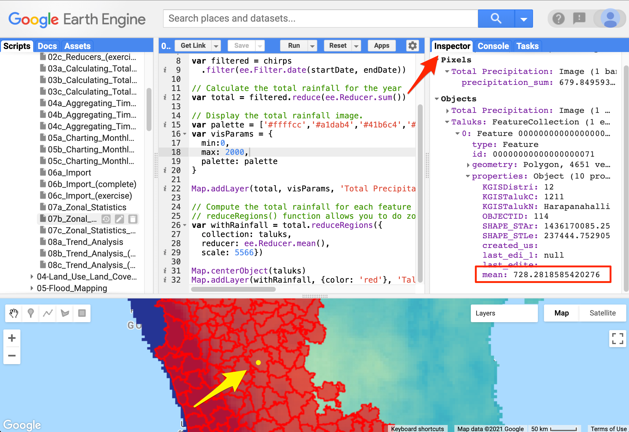
Zonal Statistics
var taluks = ee.FeatureCollection("users/ujavalgandhi/gee-water-resources/kgis_taluks");
var chirps = ee.ImageCollection('UCSB-CHG/CHIRPS/PENTAD');

var year = 2019;
var startDate = ee.Date.fromYMD(year, 1, 1);
var endDate = startDate.advance(1, 'year');

var filtered = chirps
  .filter(ee.Filter.date(startDate, endDate));

// Calculate the total rainfall for the year
var total = filtered.reduce(ee.Reducer.sum());

// Display the total rainfall image.
var palette = ['#ffffcc','#a1dab4','#41b6c4','#2c7fb8','#253494'];
var visParams = {
  min:0,
  max: 2000,
  palette: palette
};

Map.addLayer(total, visParams, 'Total Precipitation');

// Compute the average total rainfall for each feature
// reduceRegions() function allows you to do zonal stats
var withRainfall = total.reduceRegions({
  collection: taluks,
  reducer: ee.Reducer.mean(),
  scale: 5566});

Map.centerObject(taluks);
Map.addLayer(withRainfall, {color: 'red'}, 'Taluks');
Exercise
Write an export function to export the Feature Collection as a CSV file.
var taluks = ee.FeatureCollection("users/ujavalgandhi/gee-water-resources/kgis_taluks");
var chirps = ee.ImageCollection('UCSB-CHG/CHIRPS/PENTAD');

var year = 2019;
var startDate = ee.Date.fromYMD(year, 1, 1);
var endDate = startDate.advance(1, 'year')

var filtered = chirps
  .filter(ee.Filter.date(startDate, endDate));

// Calculate the total rainfall for the year
var total = filtered.reduce(ee.Reducer.sum());

// Display the total rainfall image.
var palette = ['#ffffcc','#a1dab4','#41b6c4','#2c7fb8','#253494'];
var visParams = {
  min:0,
  max: 2000,
  palette: palette
};

Map.addLayer(total, visParams, 'Total Precipitation');

// Compute the total rainfall for each feature
// reduceRegions() function allows you to do zonal stats
var withRainfall = total.reduceRegions({
  collection: taluks,
  reducer: ee.Reducer.mean(),
  scale: 5566});

Map.centerObject(taluks);
Map.addLayer(withRainfall, {color: 'blue'}, 'Taluks');

// Exercise
// Export the resulting FeatureCollection with average rainfall as a CSV
// Use the Export.table.toDrive() function

// You can use the .select() function to select only columns you need
// You can also rename the columns
var exportCol = withRainfall
  .select(['KGISTalukN', 'mean'], ['taluk', 'average_rainfall']);
print(exportCol);

// Export the exportCol as a CSV

// Hint: Even though you have only 2 properties for each feature,
// the CSV will include internal properties system:index and .geo (the geometry)
// To only get the data columns in your CSV, specify the list of properties
// using the 'selectors' argument in Export.table.toDrive() function
08. Trend Analysis
Trend Analysis is a technique that is used to find the pattern. Let us do a Non-Parametric Trend Analysis using the Sen Slope technique to find the pattern of rainfall over time.
The sens slope is a reduction operation that expects two-band X and
Y. The X is the constant band with value year, and the Y is the total
precipitation of that pixel in that year. After creating the image
collection in this format we can use the
ee.Reducer.sensSlope() with the collection to compute the
slope at each year.
This function returns an image with a positive pixel value representing the increase in precipitation and vice-versa.
An advantage of doing trend analysis in earth engine is computing pre-pixel calculation other wise which would be computation intestiive task to perform.
var taluks = ee.FeatureCollection("users/ujavalgandhi/gee-water-resources/kgis_taluks");
var chirps = ee.ImageCollection('UCSB-CHG/CHIRPS/PENTAD');

// We will compute the trend of total seasonal rainfall

// Rainy season is June - September
var createSeasonalImage = function(year) {
  var startDate = ee.Date.fromYMD(year, 6, 1);
  var endDate = ee.Date.fromYMD(year, 10, 1);
  var seasonFiltered = chirps
    .filter(ee.Filter.date(startDate, endDate));
  // Calculate total precipitation
  var total = seasonFiltered.reduce(ee.Reducer.sum());
  return total.set({
    'system:time_start': startDate.millis(),
    'system:time_end': endDate.millis(),
    'year': year,
  });
};

// Aggregate Precipitation Data to Yearly Time-Series
var years = ee.List.sequence(1981, 2013);
var yearlyImages = years.map(createSeasonalImage);
print(yearlyImages);

var yearlyCol = ee.ImageCollection.fromImages(yearlyImages);


// Prepare data for Sen's Slope Estimation
// We need an image with 2 bands for X and Y varibles
// X = year
// Y = total precipitation

var processImage = function(image) {
  var year = image.get('year');
  var yearImage = ee.Image.constant(ee.Number(year)).toShort();
  return ee.Image.cat(yearImage, image).rename(['year', 'prcp']).set('year', year);
};

var processedCol = yearlyCol.map(processImage);
print(processedCol);

// Calculate time series slope using sensSlope().
var sens = processedCol.reduce(ee.Reducer.sensSlope());

// The resulting image has 2 bands: slope and intercept
// We select the 'slope' band
var slope = sens.select('slope');
// Set visualisation parameters
var visParams = {min: -10, max: 10, palette: ['brown', 'white', 'blue']};
Map.addLayer(slope, visParams, 'Trend');
Exercise
The trend analysis is done for a particular season. Change the filter dates to compute the annual precipitation trend.
var taluks = ee.FeatureCollection("users/ujavalgandhi/gee-water-resources/kgis_taluks");
var chirps = ee.ImageCollection('UCSB-CHG/CHIRPS/PENTAD');

// We will compute the trend of total seasonal rainfall

// Rainy season is June - September
var createSeasonalImage = function(year) {
  var startDate = ee.Date.fromYMD(year, 6, 1);
  var endDate = ee.Date.fromYMD(year, 10, 1);
  var seasonFiltered = chirps
    .filter(ee.Filter.date(startDate, endDate));
  // Calculate total precipitation
  var total = seasonFiltered.reduce(ee.Reducer.sum());
  return total.set({
    'system:time_start': startDate.millis(),
    'system:time_end': endDate.millis(),
    'year': year,
  });
};

// Aggregate Precipitation Data
var years = ee.List.sequence(1981, 2013);
var yearlyImages = years.map(createSeasonalImage);
print(yearlyImages);

var yearlyCol = ee.ImageCollection.fromImages(yearlyImages);


// Prepare data for Sen's Slope Estimation
// We need an image with 2 bands for X and Y varibles
// X = year
// Y = total precipitation

var processImage = function(image) {
  var year = image.get('year');
  var yearImage = ee.Image.constant(ee.Number(year)).toShort();
  return ee.Image.cat(yearImage, image).rename(['year', 'prcp']).set('year', year);
};

var processedCol = yearlyCol.map(processImage);
print(processedCol);

// Calculate time series slope using sensSlope().
var sens = processedCol.reduce(ee.Reducer.sensSlope());

// The resulting image has 2 bands: slope and intercept
// We select the 'slope' band
var slope = sens.select('slope');
// Set visualisation parameters
var visParams = {min: -10, max: 10, palette: ['brown', 'white', 'blue']};
Map.addLayer(slope, visParams, 'Trend');

// Exercise
// Change the code above to compute annual precipitation trend
Module 4: Land Use Land Cover Classification
Supervised classification is one of the most popular machine learning technique used in remote sensing. Google Earth Engine is uniquely suited for supervised classification at a large scale and offers a flexible data model that allows you to easily incorporate variables from multiple data sources. The interactive nature of Earth Engine development allows for iterative development of supervised classification workflows by combining many different datasets into the model. This module covers basic supervised classification workflow, accuracy assessment, and area calculation.

01. Basic Supervised Classification
We will learn the technique to do a basic land cover classification
using training points collected using the Code Editor with the help of
the High-Resolution base map imagery provided by Google Maps. Even if no
field data is available for training the model, this method is very
effective in generating high-quality classification samples anywhere in
the world. The goal is to classify Sentinel 2A pixel into one of the
following classes - urban, bare, water, or vegetation.
Using the drawing tools in the code editor lets us create 4 new feature
collections with points representing pixels of each class. Each feature
collection will be created with a property landcover where
each collection has values of 0, 1, 2, or 3, representing urban, bare,
water, or vegetation, respectively. We use these collected samples to
train a Random Forest classifier and apply it to all the image
pixels to create a land cover image with 4 classes.
Fun fact: The classifiers in Earth Engine API have names starting with smile - such as
ee.Classifier.smileRandomForest(). The smile part refers to the Statistical Machine Intelligence and Learning Engine (SMILE) JAVA library which is used by Google Earth Engine to implement these algorithms.
var city = ee.FeatureCollection('projects/spatialthoughts/assets/e2e/bangalore_boundary');
var geometry = city.geometry();

var s2 = ee.ImageCollection('COPERNICUS/S2_SR_HARMONIZED');
// The following collections were created using the
// Drawing Tools in the code editor
var urban = ee.FeatureCollection('projects/spatialthoughts/assets/e2e/urban_gcps');
var bare = ee.FeatureCollection('projects/spatialthoughts/assets/e2e/bare_gcps');
var water = ee.FeatureCollection('projects/spatialthoughts/assets/e2e/water_gcps');
var vegetation = ee.FeatureCollection('projects/spatialthoughts/assets/e2e/vegetation_gcps');

var year = 2019;
var startDate = ee.Date.fromYMD(year, 1, 1);
var endDate = startDate.advance(1, 'year');

var filtered = s2
  .filter(ee.Filter.lt('CLOUDY_PIXEL_PERCENTAGE', 30))
  .filter(ee.Filter.date(startDate, endDate))
  .filter(ee.Filter.bounds(geometry));

// Load the Cloud Score+ collection
var csPlus = ee.ImageCollection('GOOGLE/CLOUD_SCORE_PLUS/V1/S2_HARMONIZED');
var csPlusBands = csPlus.first().bandNames();

// We need to add Cloud Score + bands to each Sentinel-2
// image in the collection
// This is done using the linkCollection() function
var filteredS2WithCs = filtered.linkCollection(csPlus, csPlusBands);

// Function to mask pixels with low CS+ QA scores.
function maskLowQA(image) {
  var qaBand = 'cs';
  var clearThreshold = 0.5;
  var mask = image.select(qaBand).gte(clearThreshold);
  return image.updateMask(mask);
}

var filteredMasked = filteredS2WithCs
  .map(maskLowQA)
  .select('B.*');

var composite = filteredMasked.median();

// Display the input composite.
var rgbVis = {
  min: 0.0,
  max: 3000,
  bands: ['B4', 'B3', 'B2'],
};
Map.addLayer(composite.clip(geometry), rgbVis, 'image');

var gcps = urban.merge(bare).merge(water).merge(vegetation);

// Overlay the point on the image to get training data.
var training = composite.sampleRegions({
  collection: gcps,
  properties: ['landcover'],
  scale: 10
});


// Train a classifier.
var classifier = ee.Classifier.smileRandomForest(50).train({
  features: training,
  classProperty: 'landcover',
  inputProperties: composite.bandNames()
});
// // Classify the image.
var classified = composite.classify(classifier);
// Choose a 4-color palette
// Assign a color for each class in the following order
// Urban, Bare, Water, Vegetation
var palette = ['#cc6d8f', '#ffc107', '#1e88e5', '#004d40' ];

Map.addLayer(classified.clip(geometry), {min: 0, max: 3, palette: palette}, 'Classification');

// Select the Water class
var waterClass = classified.eq(2);
var waterVis = {min:0, max:1, palette: ['white', 'blue']};
Map.addLayer(waterClass.clip(geometry), waterVis, 'Water', false);

// Display the GCPs
// We use the style() function to style the GCPs
var palette = ee.List(palette);
var landcover = ee.List([0, 1, 2, 3]);

var gcpsStyled = ee.FeatureCollection(
  landcover.map(function(lc){
    var color = palette.get(landcover.indexOf(lc));
    var markerStyle = { color: 'white', pointShape: 'diamond',
      pointSize: 4, width: 1, fillColor: color};
    return gcps.filter(ee.Filter.eq('landcover', lc))
                .map(function(point){
                  return point.set('style', markerStyle);
                });
      })).flatten();

Map.addLayer(gcpsStyled.style({styleProperty:"style"}), {}, 'GCPs');
Map.centerObject(gcpsStyled);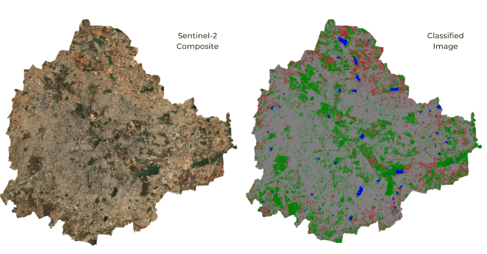
Supervised Classification Output
Exercise
Select and city of your choice from urbanAreas data.
Create Feature collection with property landcover and
collect training points for every four classes urban, bare,
water, and vegetation. Then use the code to classify and
create a land cover of the city.
// Perform supervised classification for your city

// Delete the geometry below and draw a polygon
// over your chosen city
var geometry = ee.Geometry.Polygon([[
  [77.4149, 13.1203],
  [77.4149, 12.7308],
  [77.8090, 12.7308],
  [77.8090, 13.1203]
]]);

Map.centerObject(geometry);

var year = 2019;
var startDate = ee.Date.fromYMD(year, 1, 1);
var endDate = startDate.advance(1, 'year');

var s2 = ee.ImageCollection('COPERNICUS/S2_SR_HARMONIZED');

var filtered = s2
  .filter(ee.Filter.lt('CLOUDY_PIXEL_PERCENTAGE', 30))
  .filter(ee.Filter.date(startDate, endDate))
  .filter(ee.Filter.bounds(geometry));

// Load the Cloud Score+ collection
var csPlus = ee.ImageCollection('GOOGLE/CLOUD_SCORE_PLUS/V1/S2_HARMONIZED');
var csPlusBands = csPlus.first().bandNames();

// We need to add Cloud Score + bands to each Sentinel-2
// image in the collection
// This is done using the linkCollection() function
var filteredS2WithCs = filtered.linkCollection(csPlus, csPlusBands);

// Function to mask pixels with low CS+ QA scores.
function maskLowQA(image) {
  var qaBand = 'cs';
  var clearThreshold = 0.5;
  var mask = image.select(qaBand).gte(clearThreshold);
  return image.updateMask(mask);
}

var filteredMasked = filteredS2WithCs
  .map(maskLowQA)
  .select('B.*');

var composite = filteredMasked.median();

// Display the input composite.

var rgbVis = {min: 0.0, max: 3000, bands: ['B4', 'B3', 'B2']};
Map.addLayer(composite.clip(geometry), rgbVis, 'image');

// Exercise
// Add training points for 4 classes
// Assign the 'landcover' property as follows

// urban: 0
// bare: 1
// water: 2
// vegetation: 3

// After adding points, uncomments lines below

// var gcps = urban.merge(bare).merge(water).merge(vegetation);

// // Overlay the point on the image to get training data.
// var training = composite.sampleRegions({
//   collection: gcps,
//   properties: ['landcover'],
//   scale: 10,
//   tileScale: 16
// });
// print(training);


// // Train a classifier.
// var classifier = ee.Classifier.smileRandomForest(50).train({
//   features: training,
//   classProperty: 'landcover',
//   inputProperties: composite.bandNames()
// });
// // // Classify the image.
// var classified = composite.classify(classifier);

// // Choose a 4-color palette
// // Assign a color for each class in the following order
// // Urban, Bare, Water, Vegetation
// var palette = ['#cc6d8f', '#ffc107', '#1e88e5', '#004d40' ];

// Map.addLayer(classified.clip(geometry), {min: 0, max: 3, palette: palette}, 'Classification');

// // Select the Water class
// var waterClass = classified.eq(2);
// var waterVis = {min:0, max:1, palette: ['white', 'blue']};
// Map.addLayer(waterClass.clip(geometry), waterVis, 'Water', false);
02. Accuracy Assessment
It is important to get a quantitative estimate of the accuracy of the
classification. To do this, a common strategy is to divide your training
samples into 2 random fractions - one used for training the
model and the other for validation of the predictions. Once a
classifier is trained, it can be used to classify the entire image. We
can then compare the classified values with the ones in the validation
fraction. We can use the ee.Classifier.confusionMatrix()
method to calculate a Confusion Matrix representing expected
accuracy.
Don’t get carried away tweaking your model to give you the highest validation accuracy. You must use both qualitative measures (such as visual inspection of results) along with quantitative measures to assess the results.
// Load training samples
// This was created by exporting the merged 'gcps' collection
// using Export.table.toAsset()
var gcps = ee.FeatureCollection('projects/spatialthoughts/assets/e2e/exported_gcps');

// Load the region boundary of a basin
var boundary = ee.FeatureCollection('projects/spatialthoughts/assets/e2e/basin_boundary');
var geometry = boundary.geometry();
Map.centerObject(geometry);

var rgbVis = {
  min: 0.0,
  max: 3000,
  bands: ['B4', 'B3', 'B2'],
};

var year = 2019;
var startDate = ee.Date.fromYMD(year, 1, 1);
var endDate = startDate.advance(1, 'year');

var s2 = ee.ImageCollection('COPERNICUS/S2_SR_HARMONIZED');

var filtered = s2
  .filter(ee.Filter.lt('CLOUDY_PIXEL_PERCENTAGE', 30))
  .filter(ee.Filter.date(startDate, endDate))
  .filter(ee.Filter.bounds(geometry));

// Load the Cloud Score+ collection
var csPlus = ee.ImageCollection('GOOGLE/CLOUD_SCORE_PLUS/V1/S2_HARMONIZED');
var csPlusBands = csPlus.first().bandNames();

// We need to add Cloud Score + bands to each Sentinel-2
// image in the collection
// This is done using the linkCollection() function
var filteredS2WithCs = filtered.linkCollection(csPlus, csPlusBands);

// Function to mask pixels with low CS+ QA scores.
function maskLowQA(image) {
  var qaBand = 'cs';
  var clearThreshold = 0.5;
  var mask = image.select(qaBand).gte(clearThreshold);
  return image.updateMask(mask);
}

var filteredMasked = filteredS2WithCs
  .map(maskLowQA)
  .select('B.*');

var composite = filteredMasked.median();

// Display the input composite.
Map.addLayer(composite.clip(geometry), rgbVis, 'image');


// Add a random column and split the GCPs into training and validation set
var gcps = gcps.randomColumn();

// This being a simpler classification, we take 60% points
// for validation. Normal recommended ratio is
// 70% training, 30% validation
var trainingGcp = gcps.filter(ee.Filter.lt('random', 0.6));
var validationGcp = gcps.filter(ee.Filter.gte('random', 0.6));

// Overlay the point on the image to get training data.
var training = composite.sampleRegions({
  collection: trainingGcp,
  properties: ['landcover'],
  scale: 10,
  tileScale: 16
});

// Train a classifier.
var classifier = ee.Classifier.smileRandomForest(50)
.train({
  features: training,
  classProperty: 'landcover',
  inputProperties: composite.bandNames()
});

// Classify the image.
var classified = composite.classify(classifier);

var palette = ['#cc6d8f', '#ffc107', '#1e88e5', '#004d40' ];
Map.addLayer(classified.clip(geometry), {min: 0, max: 3, palette: palette}, 'Classification');
//**************************************************************************
// Accuracy Assessment
//**************************************************************************

// Use classification map to assess accuracy using the validation fraction
// of the overall training set created above.
var test = classified.sampleRegions({
  collection: validationGcp,
  properties: ['landcover'],
  tileScale: 16,
  scale: 10,
});

var testConfusionMatrix = test.errorMatrix('landcover', 'classification');
// Printing of confusion matrix may time out. Alternatively, you can export it as CSV
print('Confusion Matrix', testConfusionMatrix);
print('Test Accuracy', testConfusionMatrix.accuracy());

// Alternate workflow
// This is similar to machine learning practice
var validation = composite.sampleRegions({
  collection: validationGcp,
  properties: ['landcover'],
  scale: 10,
  tileScale: 16
});

var test = validation.classify(classifier);

var testConfusionMatrix = test.errorMatrix('landcover', 'classification');
// Printing of confusion matrix may time out. Alternatively, you can export it as CSV
print('Confusion Matrix', testConfusionMatrix);
print('Test Accuracy', testConfusionMatrix.accuracy());
03. Feature Engineering
// Load training samples
// This was created by exporting the merged 'gcps' collection
// using Export.table.toAsset()
var gcps = ee.FeatureCollection('projects/spatialthoughts/assets/e2e/exported_gcps');

// Load the region boundary of a basin
var boundary = ee.FeatureCollection('projects/spatialthoughts/assets/e2e/basin_boundary');
var geometry = boundary.geometry();
Map.centerObject(geometry);

var rgbVis = {
  min: 0.0,
  max: 3000,
  bands: ['B4', 'B3', 'B2'],
};

var year = 2019;
var startDate = ee.Date.fromYMD(year, 1, 1);
var endDate = startDate.advance(1, 'year');

var s2 = ee.ImageCollection('COPERNICUS/S2_SR_HARMONIZED');

var filtered = s2
  .filter(ee.Filter.lt('CLOUDY_PIXEL_PERCENTAGE', 30))
  .filter(ee.Filter.date(startDate, endDate))
  .filter(ee.Filter.bounds(geometry));

// Load the Cloud Score+ collection
var csPlus = ee.ImageCollection('GOOGLE/CLOUD_SCORE_PLUS/V1/S2_HARMONIZED');
var csPlusBands = csPlus.first().bandNames();

// We need to add Cloud Score + bands to each Sentinel-2
// image in the collection
// This is done using the linkCollection() function
var filteredS2WithCs = filtered.linkCollection(csPlus, csPlusBands);

// Function to mask pixels with low CS+ QA scores.
function maskLowQA(image) {
  var qaBand = 'cs';
  var clearThreshold = 0.5;
  var mask = image.select(qaBand).gte(clearThreshold);
  return image.updateMask(mask);
}

var filteredMasked = filteredS2WithCs
  .map(maskLowQA)
  .select('B.*');

var composite = filteredMasked.median();

// Display the input composite.
Map.addLayer(composite.clip(geometry), rgbVis, 'image');

// Add New Features to the Model

// 1. Add Indices
var addIndices = function(image) {
  var ndvi = image.normalizedDifference(['B8', 'B4']).rename(['ndvi']);
  var ndbi = image.normalizedDifference(['B11', 'B8']).rename(['ndbi']);
  var mndwi = image.normalizedDifference(['B3', 'B11']).rename(['mndwi']);
  var bsi = image.expression(
      '(( X + Y ) - (A + B)) /(( X + Y ) + (A + B)) ', {
        'X': image.select('B11'), //swir1
        'Y': image.select('B4'),  //red
        'A': image.select('B8'), // nir
        'B': image.select('B2'), // blue
  }).rename('bsi');
  return image.addBands(ndvi).addBands(ndbi).addBands(mndwi).addBands(bsi);
};

var composite = addIndices(composite);

// 2. Add Slope and Elevation

// Use ALOS World 3D
var alos = ee.ImageCollection('JAXA/ALOS/AW3D30/V4_1');

// This comes as a collection of images
// We mosaic it to create a single image

// Need to set the projection correctly on the mosaic
// for the slope computation
var proj = alos.first().projection();

var elevation = alos.select('DSM').mosaic()
  .setDefaultProjection(proj)
  .rename('elev');

var slope = ee.Terrain.slope(elevation)
  .rename('slope');

var composite = composite.addBands(elevation).addBands(slope);

print('Composite Bands', composite);

// Train the model with new features

// Add a random column and split the GCPs into training and validation set
var gcps = gcps.randomColumn();

// This being a simpler classification, we take 60% points
// for validation. Normal recommended ratio is
// 70% training, 30% validation
var trainingGcp = gcps.filter(ee.Filter.lt('random', 0.6));
var validationGcp = gcps.filter(ee.Filter.gte('random', 0.6));

// Overlay the point on the image to get training data.
var training = composite.sampleRegions({
  collection: trainingGcp,
  properties: ['landcover'],
  scale: 10,
  tileScale: 16
});

print('Training Feature', training.first());

// Train a classifier.
var classifier = ee.Classifier.smileRandomForest(50)
.train({
  features: training,
  classProperty: 'landcover',
  inputProperties: composite.bandNames()
});

// Classify the image.
var classified = composite.classify(classifier);

var palette = ['#cc6d8f', '#ffc107', '#1e88e5', '#004d40' ];
Map.addLayer(classified.clip(geometry), {min: 0, max: 3, palette: palette}, 'Classification');
//**************************************************************************
// Accuracy Assessment
//**************************************************************************

// Use classification map to assess accuracy using the validation fraction
// of the overall training set created above.
var test = classified.sampleRegions({
  collection: validationGcp,
  properties: ['landcover'],
  tileScale: 16,
  scale: 10,
});

var testConfusionMatrix = test.errorMatrix('landcover', 'classification');
// Printing of confusion matrix may time out. Alternatively, you can export it as CSV
print('Confusion Matrix', testConfusionMatrix);
print('Test Accuracy', testConfusionMatrix.accuracy());
Exercise
// Exercise

// Improve your classification from Exercise 01c

// Add new features to your model using the code below
// to your own classification

// Copy the block of code at the end of your script

// ******** Start Copy/Paste ************

// Add New Features to the Model
var addIndices = function(image) {
  var ndvi = image.normalizedDifference(['B8', 'B4']).rename(['ndvi']);
  var ndbi = image.normalizedDifference(['B11', 'B8']).rename(['ndbi']);
  var mndwi = image.normalizedDifference(['B3', 'B11']).rename(['mndwi']);
  var bsi = image.expression(
      '(( X + Y ) - (A + B)) /(( X + Y ) + (A + B)) ', {
        'X': image.select('B11'), //swir1
        'Y': image.select('B4'),  //red
        'A': image.select('B8'), // nir
        'B': image.select('B2'), // blue
  }).rename('bsi');
  return image.addBands(ndvi).addBands(ndbi).addBands(mndwi).addBands(bsi);
};

var composite = addIndices(composite);

// Calculate Slope and Elevation

// Use ALOS World 3D
var alos = ee.ImageCollection('JAXA/ALOS/AW3D30/V4_1');

// This comes as a collection of images
// We mosaic it to create a single image

// Need to set the projection correctly on the mosaic
// for the slope computation
var proj = alos.first().projection();

var elevation = alos.select('DSM').mosaic()
  .setDefaultProjection(proj)
  .rename('elev');

var slope = ee.Terrain.slope(elevation)
  .rename('slope');

var composite = composite.addBands(elevation).addBands(slope);

// Overlay the point on the image to get training data.
var training = composite.sampleRegions({
  collection: gcps,
  properties: ['landcover'],
  scale: 10
});


// Train a classifier.
var classifier = ee.Classifier.smileRandomForest(50).train({
  features: training,
  classProperty: 'landcover',
  inputProperties: composite.bandNames()
});
// // Classify the image.
var classified = composite.classify(classifier);
Map.addLayer(classified.clip(geometry), {min: 0, max: 3, palette: palette}, 'Classification (S2 + Features)');

// Select the Water class
var waterClass = classified.eq(2);
var waterVis = {min:0, max:1, palette: ['white', 'blue']};
Map.addLayer(waterClass.clip(geometry), waterVis, 'Water (S2 + Features)', false);

// ********** End Copy/Paste  *************
04. Using Satellite Embeddings
Satellite Embedding is a wew global dataset produced by Google DeepMind’s AlphaEarth Foundations model. The model ingests time-series of many different earth observation datasets to produce a unified digital representation of each pixel - called embeddings. The embeddings are provided as an analysis-ready dataset in Earth Engine with yearly images from 2017-current. Embeddings can be used as input features to the classification model and results in higher accuracy outputs.
// Load training samples
// This was created by exporting the merged 'gcps' collection
// using Export.table.toAsset()
var gcps = ee.FeatureCollection('projects/spatialthoughts/assets/e2e/exported_gcps');

// Load the region boundary of a basin
var boundary = ee.FeatureCollection('projects/spatialthoughts/assets/e2e/basin_boundary');
var geometry = boundary.geometry();
Map.centerObject(geometry);

var rgbVis = {
  min: 0.0,
  max: 3000,
  bands: ['B4', 'B3', 'B2'],
};

var year = 2019;
var startDate = ee.Date.fromYMD(year, 1, 1);
var endDate = startDate.advance(1, 'year');

var s2 = ee.ImageCollection('COPERNICUS/S2_SR_HARMONIZED');

var filtered = s2
  .filter(ee.Filter.lt('CLOUDY_PIXEL_PERCENTAGE', 30))
  .filter(ee.Filter.date(startDate, endDate))
  .filter(ee.Filter.bounds(geometry));

// Load the Cloud Score+ collection
var csPlus = ee.ImageCollection('GOOGLE/CLOUD_SCORE_PLUS/V1/S2_HARMONIZED');
var csPlusBands = csPlus.first().bandNames();

// We need to add Cloud Score + bands to each Sentinel-2
// image in the collection
// This is done using the linkCollection() function
var filteredS2WithCs = filtered.linkCollection(csPlus, csPlusBands);

// Function to mask pixels with low CS+ QA scores.
function maskLowQA(image) {
  var qaBand = 'cs';
  var clearThreshold = 0.5;
  var mask = image.select(qaBand).gte(clearThreshold);
  return image.updateMask(mask);
}

var filteredMasked = filteredS2WithCs
  .map(maskLowQA)
  .select('B.*');

var composite = filteredMasked.median();

// Display the input composite.
Map.addLayer(composite.clip(geometry), rgbVis, 'image');

// Use Satellite Embeddings as Features

var embeddings = ee.ImageCollection('GOOGLE/SATELLITE_EMBEDDING/V1/ANNUAL');

var filteredEmbeddings = embeddings
  .filter(ee.Filter.date(startDate, endDate))
  .filter(ee.Filter.bounds(geometry));

var embeddingsImage = filteredEmbeddings.mosaic();
print('Satellite Embedding Image', embeddingsImage);

// Train a classifier.

// Add a random column and split the GCPs into training and validation set
var gcps = gcps.randomColumn();

// This being a simpler classification, we take 60% points
// for validation. Normal recommended ratio is
// 70% training, 30% validation
var trainingGcp = gcps.filter(ee.Filter.lt('random', 0.6));
var validationGcp = gcps.filter(ee.Filter.gte('random', 0.6));

// Overlay the point on the image to get training data.
var training = embeddingsImage.sampleRegions({
  collection: trainingGcp,
  properties: ['landcover'],
  scale: 10,
  tileScale: 16
});

print('Training Feature', training.first());

var classifier = ee.Classifier.smileKNN()
.train({
  features: training,
  classProperty: 'landcover',
  inputProperties: embeddingsImage.bandNames()
});

// Classify the image.
var classified = embeddingsImage.classify(classifier);

var palette = ['#cc6d8f', '#ffc107', '#1e88e5', '#004d40' ];
Map.addLayer(classified.clip(geometry), {min: 0, max: 3, palette: palette}, 'Classification');
//**************************************************************************
// Accuracy Assessment
//**************************************************************************

// Use classification map to assess accuracy using the validation fraction
// of the overall training set created above.
var test = classified.sampleRegions({
  collection: validationGcp,
  properties: ['landcover'],
  tileScale: 16,
  scale: 10,
});

var testConfusionMatrix = test.errorMatrix('landcover', 'classification');
// Printing of confusion matrix may time out. Alternatively, you can export it as CSV
print('Confusion Matrix', testConfusionMatrix);
print('Test Accuracy', testConfusionMatrix.accuracy());
Exercise
// Exercise

// Improve your classification from Exercise 01c

// Use satellite embeddings as features
// for your own classification

// Copy the block of code at the end of your script

// ******** Start Copy/Paste ************

// Use Satellite Embeddings as Features

var embeddings = ee.ImageCollection('GOOGLE/SATELLITE_EMBEDDING/V1/ANNUAL');

var filteredEmbeddings = embeddings
  .filter(ee.Filter.date(startDate, endDate))
  .filter(ee.Filter.bounds(geometry));

var embeddingsImage = filteredEmbeddings.mosaic();
print('Satellite Embedding Image', embeddingsImage);

var gcps = urban.merge(bare).merge(water).merge(vegetation);

// Overlay the point on the image to get training data.
var training = embeddingsImage.sampleRegions({
  collection: gcps,
  properties: ['landcover'],
  scale: 10
});

print(training.first());

// Train a classifier.
var classifier = ee.Classifier.smileKNN().train({
  features: training,
  classProperty: 'landcover',
  inputProperties: embeddingsImage.bandNames()
});

// Classify the image.
var classified = embeddingsImage.classify(classifier);
Map.centerObject(geometry);
// Choose a 4-color palette
// Assign a color for each class in the following order
// Urban, Bare, Water, Vegetation
var palette = ['#cc6d8f', '#ffc107', '#1e88e5', '#004d40' ];

Map.addLayer(classified.clip(geometry), {min: 0, max: 3, palette: palette},
  'Classification (Embeddings)');

// Select the Water class
var waterClass = classified.eq(2);
var waterVis = {min:0, max:1, palette: ['white', 'blue']};
Map.addLayer(waterClass.clip(geometry), waterVis, 'Water (Embeddings)', false);

// ******** End Copy/Paste ************
05. Using Existing Landcover Datasets
One of the ambitious projects was creating a global landcover data with many classes for many years. This type of data is essential as in expect few countries, the landcover data of terrain is not available / not shared publicly by the local governments. Hence creating a global land cover has been attempted by a few organizations One among them is European Space Agency. The ESA has created the 10m global landcover called WorldCover with 10 classes. At present, this data is available for the year 2020 and, ESA has promised to develop and release this data every year following 2020. Watch the launch event to know more about this data and the methodology used to create this.
We can use the eq operator to extract a particular
class, extract the water class, and create a surface water map for the
Arkavathy region.
var dataset = ee.ImageCollection("ESA/WorldCover/v100").first();

// Select a Basin
var basin = ee.FeatureCollection("WWF/HydroSHEDS/v1/Basins/hybas_7");
var selected = basin.filter(ee.Filter.eq('HYBAS_ID', 4071139640))
var geometry = selected.geometry()

Map.centerObject(geometry);
// Add the classified image
var classification = dataset.select('Map').clip(geometry)

Map.addLayer(classification, {}, 'WorldCover Classification')
// Select water class
var water = classification.eq(80)
Map.addLayer(water, {min:0, max:1, palette: ['white', 'blue']}, 'Water')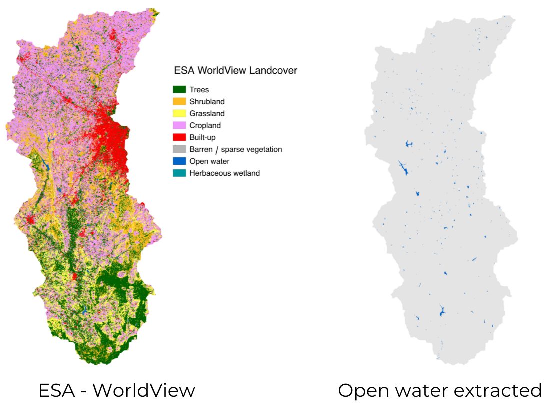
WorldView
Exercise
Use the WorldCover data and extract the Cropland class
for Arkavathy region. Then add it to map with green
palette.
var dataset = ee.ImageCollection("ESA/WorldCover/v100").first();

// Select a Basin
var basin = ee.FeatureCollection("WWF/HydroSHEDS/v1/Basins/hybas_7");
var selected = basin.filter(ee.Filter.eq('HYBAS_ID', 4071139640))
var geometry = selected.geometry()

Map.centerObject(geometry);
// Add the classified image
var classification = dataset.select('Map').clip(geometry)

Map.addLayer(classification, {}, 'WorldCover Classification')

// Change the region to a basin of your choice
// Extract the 'Cropland' class
// Apply a selfMask()
// Add it to the map with the 'green' palette
06. Calculating Area
Now that we have extracted the open water from WorldCover, we will
learn how to calculate the area for pixels in each class. Calculating
area for features is done using the area() function and for
images using the ee.Image.pixelArea() function. The
ee.Image.pixelArea() function creates an image where each
pixel’s value is the area of the pixel. We multiply this pixel area
image with our image and sum up the area using the
reduceRegion() function.
The
ee.Image.pixelArea()function uses a custom equal-area projection for area calculation. The result is area in square meters regardless of the projection of the input image. Learn more
var dataset = ee.ImageCollection("ESA/WorldCover/v100").first();

// Select a Basin
var basin = ee.FeatureCollection("WWF/HydroSHEDS/v1/Basins/hybas_7");
var selected = basin.filter(ee.Filter.eq('HYBAS_ID', 4071139640));
var geometry = selected.geometry();

Map.centerObject(geometry);
// Add the classified image
var classification = dataset.select('Map').clip(geometry);

Map.addLayer(classification, {}, 'WorldCover Classification');

// .area() function calculates the area in square meters
var basinArea = geometry.area();

// We can cast the result to a ee.Number() and calculate the
// area in square kilometers
var basinAreaSqKm = ee.Number(basinArea).divide(1e6).round();
print(basinAreaSqKm);


// Area Calculation for Images
// Extract all water pixels
var water = classification.eq(80);

// If the image contains values 0 or 1, we can calculate the
// total area using reduceRegion() function

// The result of .eq() operation is a binary image with pixels
// values of 1 where the condition matched and 0 where it didn't
Map.addLayer(water, {min:0, max:1, palette: ['white', 'blue']}, 'Surface Water');

// Since our image has only 0 and 1 pixel values, the water
// pixels will have values equal to their area
var areaImage = water.multiply(ee.Image.pixelArea());


// Now that each pixel for water class in the image has the value
// equal to its area, we can sum up all the values in the region
// to get the total green cover.

var area = areaImage.reduceRegion({
  reducer: ee.Reducer.sum(),
  geometry: geometry,
  scale: 10,
  maxPixels: 1e10
});

// The result of the reduceRegion() function is a dictionary with the key
// being the band name. We can extract the area number and convert it to
// square kilometers
var waterAreaSqKm = ee.Number(area.get('Map')).divide(1e6).round();
print(waterAreaSqKm);
Output
Total basin Area(sqkm)
4178

Total water area in the basin(sqkm)
19
Exercise
Extract the area value as a number and convert it as hectares.
var dataset = ee.ImageCollection("ESA/WorldCover/v100").first();

// Select a Basin
var basin = ee.FeatureCollection("WWF/HydroSHEDS/v1/Basins/hybas_7");
var selected = basin.filter(ee.Filter.eq('HYBAS_ID', 4071139640));
var geometry = selected.geometry();

Map.centerObject(geometry);
// Add the classified image
var classification = dataset.select('Map').clip(geometry);

Map.addLayer(classification, {}, 'WorldCover Classification');

var basinArea = geometry.area();

var cropland = classification.eq(40);
Map.addLayer(cropland, {min:0, max:1, palette: ['white', 'green']}, 'Cropland');

// Since our image has only 0 and 1 pixel values, the vegetation
// pixels will have values equal to their area
var areaImage = cropland.multiply(ee.Image.pixelArea());

var area = areaImage.reduceRegion({
  reducer: ee.Reducer.sum(),
  geometry: geometry,
  scale: 10,
  maxPixels: 1e10
  });
print('Cropland Area Sq Meters', area);

// Extract the area value from the dictionaty
// Print the cropland area in hectares
// Hint: 1 Hectare = 10000 sq. meters
Module 5: Flood Mapping
This module covers the change detection techniques for mapping floods. We will work with Sentinel-1 dataset and calculate the flooded area during the 2018 Kerala Floods in Ernakulam district in India.
Sentinel-1 is an active remote sensing platform that uses the microwave C-band to collect data. The main advantage of using microwave data is that it can penetrate through clouds and capture reflectance value both day and night since it is not dependent on Sunlight for reflectance. The spatial resolution of this data is 10m, and the temporal resolution varies between 6-12 days, depending on the location.

01. Load and Filter Sentinel-1 Data
We have learned basic skills to search for a dataset and filter it to a date range and location. Let us load the Sentinel-1 C-band SAR log scaling dataset and filter the collection to flooding event time period. Filter the collection to the Ernakulam region.
Each image will have 3 bands VV, VH, and angle. Most research results say VH - (vertical transmit and horizontal receive) is best for detecting floods as water has low reflectance in the VH band and is easy to detect. Lets us select the VH band, clip it to the ROI and display it in Map with the appropriate visualization parameter.
// On 16 August 2018, severe floods affected the south Indian state Kerala
// due to unusually high rainfall during the monsoon season.
// It was the worst flood in Kerala in nearly a century.
// https://en.wikipedia.org/wiki/2018_Kerala_floods
// Select images by predefined dates
var beforeStart = '2018-07-15';
var beforeEnd = '2018-08-10';
var afterStart = '2018-08-10';
var afterEnd = '2018-08-23';

var admin2 = ee.FeatureCollection("FAO/GAUL_SIMPLIFIED_500m/2015/level2");
var ernakulam = admin2.filter(ee.Filter.eq('ADM2_NAME', 'Ernakulam'));
var geometry = ernakulam.geometry();

Map.centerObject(geometry);
Map.addLayer(geometry, {color: 'grey'}, 'Ernakulam District');

var collection= ee.ImageCollection('COPERNICUS/S1_GRD')
  .filter(ee.Filter.date(beforeStart, beforeEnd))
  .filter(ee.Filter.bounds(geometry));

var image = ee.Image(collection.first());
var imageVh = image.select('VH').clip(geometry);

Map.addLayer(imageVh, {min:-30, max: 0}, 'VH (dB)');
Exercise
To detect the flooded regions, we need 2 collections, one before and another after flood occurrence. A before image and an after image has been created. Select the VH band from the images and add both images to the map canvas.
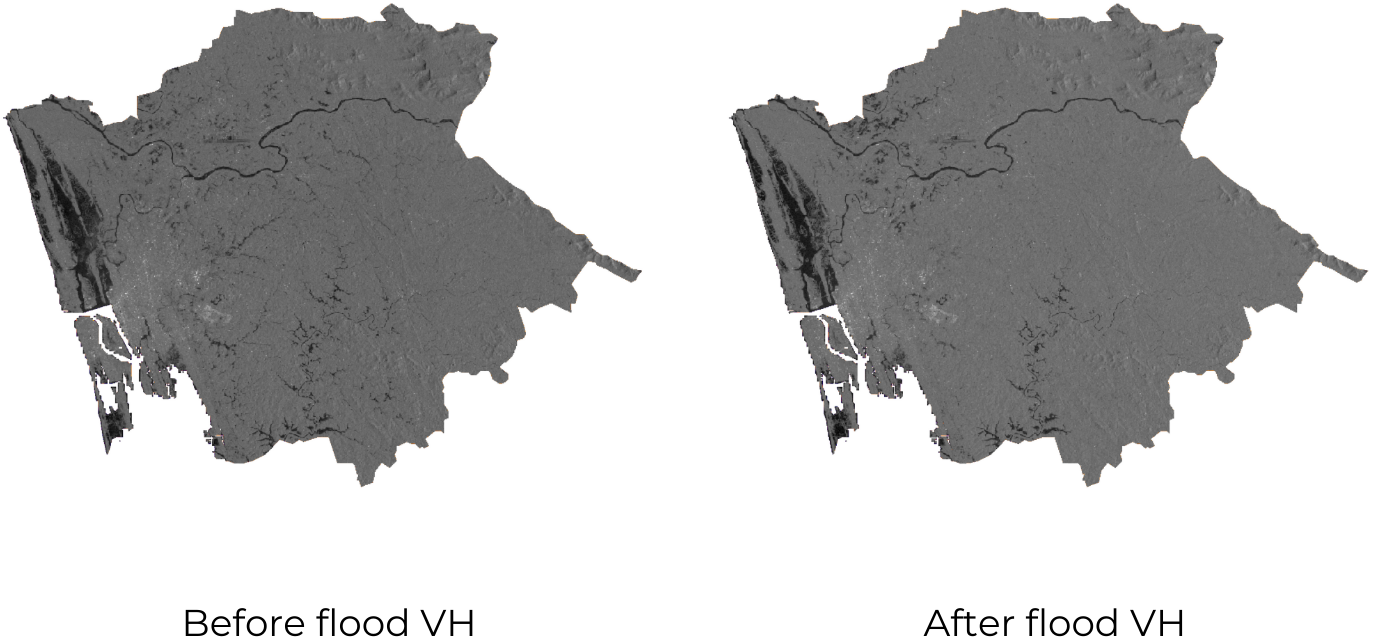
VH single band visualization
// On 16 August 2018, severe floods affected the south Indian state Kerala
// due to unusually high rainfall during the monsoon season.
// It was the worst flood in Kerala in nearly a century.
// https://en.wikipedia.org/wiki/2018_Kerala_floods
// Select images by predefined dates
var beforeStart = '2018-07-15';
var beforeEnd = '2018-08-10';
var afterStart = '2018-08-10';
var afterEnd = '2018-08-23';

var admin2 = ee.FeatureCollection("FAO/GAUL_SIMPLIFIED_500m/2015/level2");
var ernakulam = admin2.filter(ee.Filter.eq('ADM2_NAME', 'Ernakulam'));
var geometry = ernakulam.geometry();

Map.centerObject(geometry);
Map.addLayer(geometry, {color: 'grey'}, 'Ernakulam District');

var collection= ee.ImageCollection('COPERNICUS/S1_GRD')
  .filter(ee.Filter.bounds(geometry));

var beforeCollection = collection.filterDate(beforeStart, beforeEnd);
var afterCollection = collection.filterDate(afterStart,afterEnd);

var beforeImage = ee.Image(beforeCollection.first());
var afterImage = ee.Image(afterCollection.first());

print(beforeImage);
print(afterImage);
// Exercise
// Select the 'VH' band of before and after images
// Add them to the map.
// Inspect the images and find suitable values for visualization parameters
02. Visualize RGB Composites
We visualized the VH band as a single band image in the previous exercise. We can also visualize a SAR image as a multi-band RGB image. The usual practice is using the VV band in the red channel, the VH band in the green channel, and the VV/VH in the blue channel.
Three bands have different min-max values, but a single number for min-max value in visualization will not be correct. So we can pass a list of numbers, each representing each band’s min-max value in Red Green Blue order, respectively.
Open in Code Editor ↗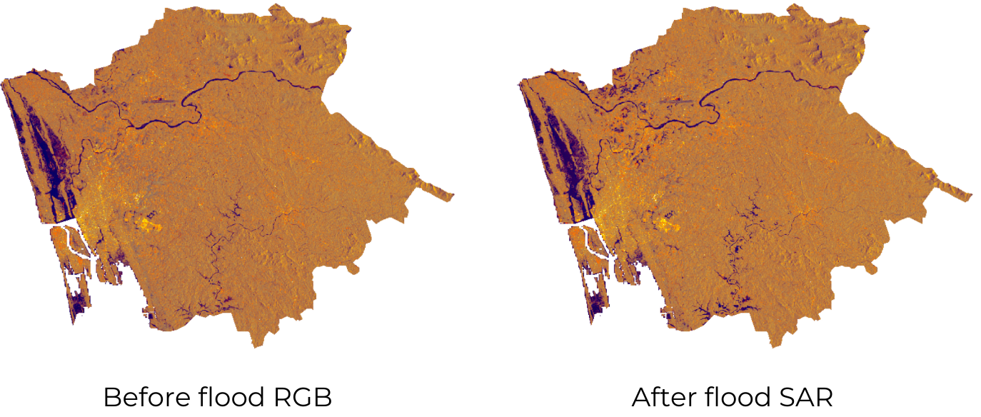
RGB multi band visualization
// On 16 August 2018, severe floods affected the south Indian state Kerala
// due to unusually high rainfall during the monsoon season.
// It was the worst flood in Kerala in nearly a century.
// https://en.wikipedia.org/wiki/2018_Kerala_floods
// Select images by predefined dates
var beforeStart = '2018-07-15';
var beforeEnd = '2018-08-10';
var afterStart = '2018-08-10';
var afterEnd = '2018-08-23';

var admin2 = ee.FeatureCollection("FAO/GAUL_SIMPLIFIED_500m/2015/level2");
var ernakulam = admin2.filter(ee.Filter.eq('ADM2_NAME', 'Ernakulam'));
var geometry = ernakulam.geometry();

Map.addLayer(geometry, {color: 'grey'}, 'Ernakulam District');

var collection= ee.ImageCollection('COPERNICUS/S1_GRD')
  .filter(ee.Filter.eq('instrumentMode','IW'))
  .filter(ee.Filter.listContains('transmitterReceiverPolarisation', 'VH'))
  .filter(ee.Filter.listContains('transmitterReceiverPolarisation', 'VV'))
  .filter(ee.Filter.eq('orbitProperties_pass', 'DESCENDING'))
  .filter(ee.Filter.eq('resolution_meters',10))
  .filter(ee.Filter.bounds(geometry))
  .select(['VV', 'VH']);

var beforeCollection = collection
  .filter(ee.Filter.date(beforeStart, beforeEnd));

var afterCollection = collection
  .filter(ee.Filter.date(afterStart, afterEnd));

var before = beforeCollection.mosaic().clip(geometry);
var after = afterCollection.mosaic().clip(geometry);

var addRatioBand = function(image) {
  var ratioBand = image.select('VV').divide(image.select('VH')).rename('VV/VH');
  return image.addBands(ratioBand);
};

var beforeRgb = addRatioBand(before);
var afterRgb = addRatioBand(after);

var visParams = {min:[-25, -25, 0] ,max:[0, 0, 2]};

Map.centerObject(geometry, 10);
Map.addLayer(beforeRgb, visParams, 'Before Floods');
Map.addLayer(afterRgb, visParams, 'After Floods');
Exercise
We have learned to visualize a multi-band image using VV, VH, and VV/VH bands. Let us visualize the change by creating a composite image with VH - before image, VH - after image, and VH - before image. This visualization can effectively identify the before and after images’ changes.
To create this visualization, select the particular bands from each
image and concatenate the three bands in the same order using
ee.Image.cat function, use the visualization parameter as
min: -25 and max: -8 and add it to the canvas.
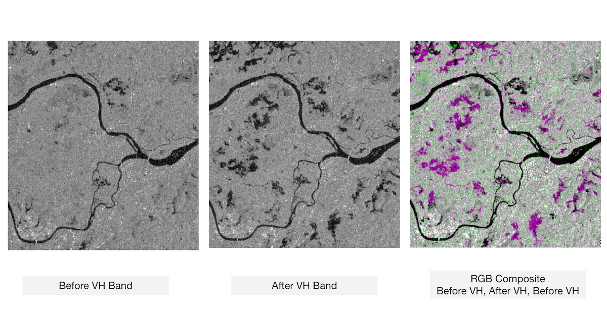
Change visualization
// On 16 August 2018, severe floods affected the south Indian state Kerala
// due to unusually high rainfall during the monsoon season.
// It was the worst flood in Kerala in nearly a century.
// https://en.wikipedia.org/wiki/2018_Kerala_floods
// Select images by predefined dates
var beforeStart = '2018-07-15';
var beforeEnd = '2018-08-10';
var afterStart = '2018-08-10';
var afterEnd = '2018-08-23';

var admin2 = ee.FeatureCollection("FAO/GAUL_SIMPLIFIED_500m/2015/level2");
var ernakulam = admin2.filter(ee.Filter.eq('ADM2_NAME', 'Ernakulam'));
var geometry = ernakulam.geometry();

Map.addLayer(geometry, {color: 'grey'}, 'Ernakulam District');

var collection= ee.ImageCollection('COPERNICUS/S1_GRD')
  .filter(ee.Filter.eq('instrumentMode','IW'))
  .filter(ee.Filter.listContains('transmitterReceiverPolarisation', 'VH'))
  .filter(ee.Filter.listContains('transmitterReceiverPolarisation', 'VV'))
  .filter(ee.Filter.eq('orbitProperties_pass', 'DESCENDING'))
  .filter(ee.Filter.eq('resolution_meters',10))
  .filter(ee.Filter.bounds(geometry))
  .select(['VV', 'VH']);

var beforeCollection = collection
  .filter(ee.Filter.date(beforeStart, beforeEnd));

var afterCollection = collection
  .filter(ee.Filter.date(afterStart, afterEnd));

var before = beforeCollection.mosaic().clip(geometry);
var after = afterCollection.mosaic().clip(geometry);

var visParams = {min: -30, max: 0};

Map.centerObject(geometry, 10);
Map.addLayer(before.select('VH'), visParams, 'Before Floods');
Map.addLayer(after.select('VH'), visParams, 'After Floods');

// Change Detection  RGB Visualization
// Create a RGB composite with following Band Combination
// Before VH, After VH, Before VH
// Hint: Use .select() to select specific band from an image
// Hint: Use ee.Image.cat() to create a 3-band image


// Display the image with a min/max range of -25 to -8
03. Apply Speckle Filter
Any SAR image will be with noise. Speckle is like salt and pepper noise in the image. Before performing any operation, a filter is applied over the image to smooth it and reduce the noise. There are many types of filters. Refined Lee filter is a more scientific approach in filtering the noise.
The raw image should be passed into the Refined Lee
function. Hence, the log image is converted to raw using the
toNatural function. The resulting image from Refined Lee is
again converted to log scale by passing it toDB
function.
Open in Code Editor ↗Guido Lemoine implemented the Refined Lee filter in GEE. Keeping the Speckle filtering function at the end of any SAR processing script can be very handy for conversions and save time.
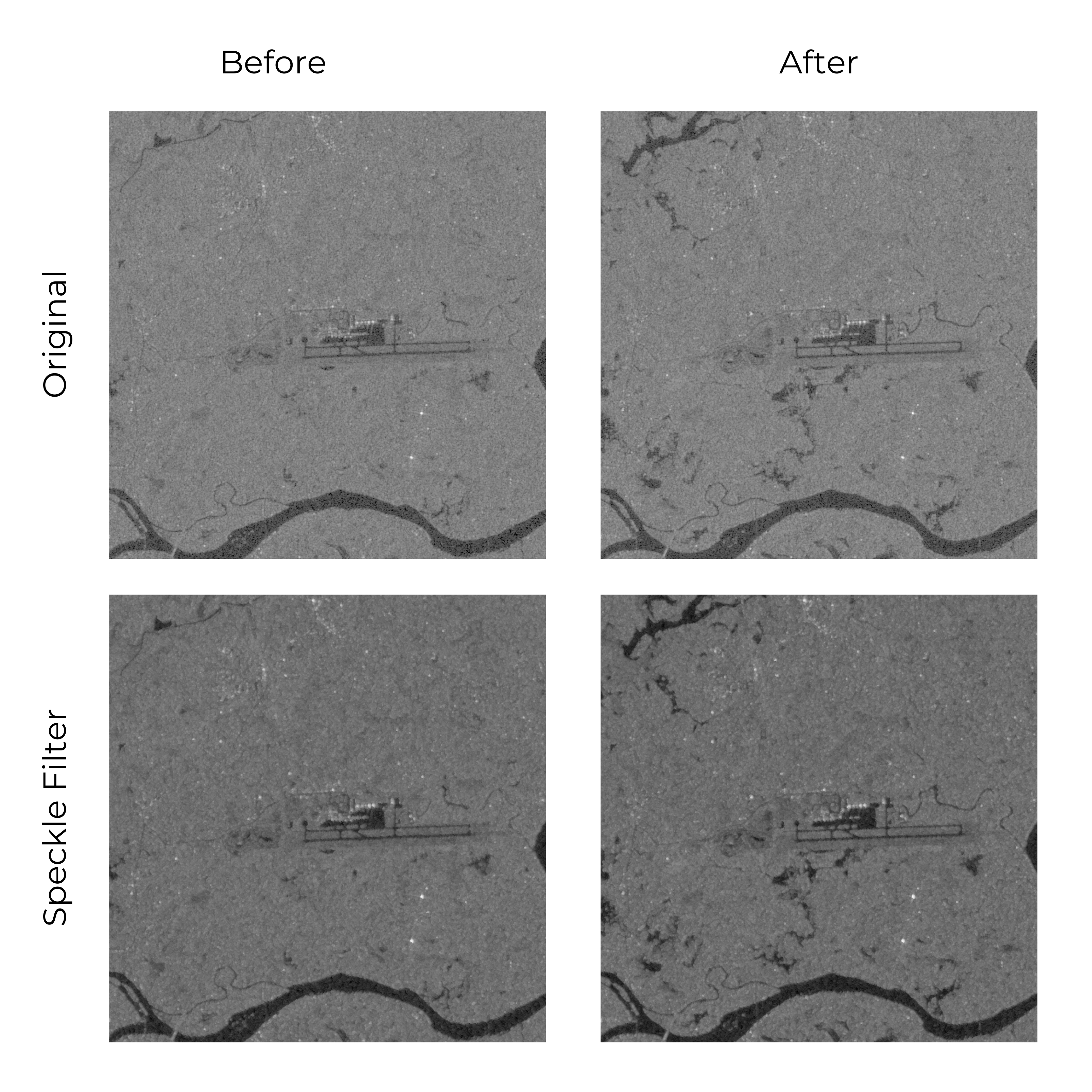
Speckle Filter
var gsw = ee.Image("JRC/GSW1_2/GlobalSurfaceWater");
var admin2 = ee.FeatureCollection("FAO/GAUL_SIMPLIFIED_500m/2015/level2");
var hydrosheds = ee.Image("WWF/HydroSHEDS/03VFDEM");

var beforeStart = '2018-07-15';
var beforeEnd = '2018-08-10';
var afterStart = '2018-08-10';
var afterEnd = '2018-08-23';

var ernakulam = admin2.filter(ee.Filter.eq('ADM2_NAME', 'Ernakulam'));
var geometry = ernakulam.geometry();
Map.addLayer(geometry, {color: 'grey'}, 'Ernakulam District');

var collection= ee.ImageCollection('COPERNICUS/S1_GRD')
  .filter(ee.Filter.eq('instrumentMode','IW'))
  .filter(ee.Filter.listContains('transmitterReceiverPolarisation', 'VH'))
  .filter(ee.Filter.eq('orbitProperties_pass', 'DESCENDING'))
  .filter(ee.Filter.eq('resolution_meters',10))
  .filter(ee.Filter.bounds(geometry))
  .select('VH');

var beforeCollection = collection
  .filter(ee.Filter.date(beforeStart, beforeEnd));

var afterCollection = collection
  .filter(ee.Filter.date(afterStart, afterEnd));

var before = beforeCollection.mosaic().clip(geometry);
var after = afterCollection.mosaic().clip(geometry);

var beforeFiltered = ee.Image(toDB(RefinedLee(toNatural(before))));
var afterFiltered = ee.Image(toDB(RefinedLee(toNatural(after))));

Map.centerObject(geometry, 10);
Map.addLayer(before, {min:-25,max:0}, 'Before Floods', false);
Map.addLayer(after, {min:-25,max:0}, 'After Floods', false);
Map.addLayer(beforeFiltered, {min:-25,max:0}, 'Before Filtered', false);
Map.addLayer(afterFiltered, {min:-25,max:0}, 'After Filtered', false);

//############################
// Speckle Filtering Functions
//############################

// Function to convert from dB
function toNatural(img) {
  return ee.Image(10.0).pow(img.select(0).divide(10.0));
}

//Function to convert to dB
function toDB(img) {
  return ee.Image(img).log10().multiply(10.0);
}

//Apllying a Refined Lee Speckle filter as coded in the SNAP 3.0 S1TBX:

//https://github.com/senbox-org/s1tbx/blob/master/s1tbx-op-sar-processing/src/main/java/org/esa/s1tbx/sar/gpf/filtering/SpeckleFilters/RefinedLee.java
//Adapted by Guido Lemoine

// by Guido Lemoine
function RefinedLee(img) {
  // img must be in natural units, i.e. not in dB!
  // Set up 3x3 kernels
  var weights3 = ee.List.repeat(ee.List.repeat(1,3),3);
  var kernel3 = ee.Kernel.fixed(3,3, weights3, 1, 1, false);

  var mean3 = img.reduceNeighborhood(ee.Reducer.mean(), kernel3);
  var variance3 = img.reduceNeighborhood(ee.Reducer.variance(), kernel3);

  // Use a sample of the 3x3 windows inside a 7x7 windows to determine gradients and directions
  var sample_weights = ee.List([[0,0,0,0,0,0,0], [0,1,0,1,0,1,0],[0,0,0,0,0,0,0], [0,1,0,1,0,1,0], [0,0,0,0,0,0,0], [0,1,0,1,0,1,0],[0,0,0,0,0,0,0]]);

  var sample_kernel = ee.Kernel.fixed(7,7, sample_weights, 3,3, false);

  // Calculate mean and variance for the sampled windows and store as 9 bands
  var sample_mean = mean3.neighborhoodToBands(sample_kernel);
  var sample_var = variance3.neighborhoodToBands(sample_kernel);

  // Determine the 4 gradients for the sampled windows
  var gradients = sample_mean.select(1).subtract(sample_mean.select(7)).abs();
  gradients = gradients.addBands(sample_mean.select(6).subtract(sample_mean.select(2)).abs());
  gradients = gradients.addBands(sample_mean.select(3).subtract(sample_mean.select(5)).abs());
  gradients = gradients.addBands(sample_mean.select(0).subtract(sample_mean.select(8)).abs());

  // And find the maximum gradient amongst gradient bands
  var max_gradient = gradients.reduce(ee.Reducer.max());

  // Create a mask for band pixels that are the maximum gradient
  var gradmask = gradients.eq(max_gradient);

  // duplicate gradmask bands: each gradient represents 2 directions
  gradmask = gradmask.addBands(gradmask);

  // Determine the 8 directions
  var directions = sample_mean.select(1).subtract(sample_mean.select(4)).gt(sample_mean.select(4).subtract(sample_mean.select(7))).multiply(1);
  directions = directions.addBands(sample_mean.select(6).subtract(sample_mean.select(4)).gt(sample_mean.select(4).subtract(sample_mean.select(2))).multiply(2));
  directions = directions.addBands(sample_mean.select(3).subtract(sample_mean.select(4)).gt(sample_mean.select(4).subtract(sample_mean.select(5))).multiply(3));
  directions = directions.addBands(sample_mean.select(0).subtract(sample_mean.select(4)).gt(sample_mean.select(4).subtract(sample_mean.select(8))).multiply(4));
  // The next 4 are the not() of the previous 4
  directions = directions.addBands(directions.select(0).not().multiply(5));
  directions = directions.addBands(directions.select(1).not().multiply(6));
  directions = directions.addBands(directions.select(2).not().multiply(7));
  directions = directions.addBands(directions.select(3).not().multiply(8));

  // Mask all values that are not 1-8
  directions = directions.updateMask(gradmask);

  // "collapse" the stack into a singe band image (due to masking, each pixel has just one value (1-8) in it's directional band, and is otherwise masked)
  directions = directions.reduce(ee.Reducer.sum());

  //var pal = ['ffffff','ff0000','ffff00', '00ff00', '00ffff', '0000ff', 'ff00ff', '000000'];
  //Map.addLayer(directions.reduce(ee.Reducer.sum()), {min:1, max:8, palette: pal}, 'Directions', false);

  var sample_stats = sample_var.divide(sample_mean.multiply(sample_mean));

  // Calculate localNoiseVariance
  var sigmaV = sample_stats.toArray().arraySort().arraySlice(0,0,5).arrayReduce(ee.Reducer.mean(), [0]);

  // Set up the 7*7 kernels for directional statistics
  var rect_weights = ee.List.repeat(ee.List.repeat(0,7),3).cat(ee.List.repeat(ee.List.repeat(1,7),4));

  var diag_weights = ee.List([[1,0,0,0,0,0,0], [1,1,0,0,0,0,0], [1,1,1,0,0,0,0],
    [1,1,1,1,0,0,0], [1,1,1,1,1,0,0], [1,1,1,1,1,1,0], [1,1,1,1,1,1,1]]);

  var rect_kernel = ee.Kernel.fixed(7,7, rect_weights, 3, 3, false);
  var diag_kernel = ee.Kernel.fixed(7,7, diag_weights, 3, 3, false);

  // Create stacks for mean and variance using the original kernels. Mask with relevant direction.
  var dir_mean = img.reduceNeighborhood(ee.Reducer.mean(), rect_kernel).updateMask(directions.eq(1));
  var dir_var = img.reduceNeighborhood(ee.Reducer.variance(), rect_kernel).updateMask(directions.eq(1));

  dir_mean = dir_mean.addBands(img.reduceNeighborhood(ee.Reducer.mean(), diag_kernel).updateMask(directions.eq(2)));
  dir_var = dir_var.addBands(img.reduceNeighborhood(ee.Reducer.variance(), diag_kernel).updateMask(directions.eq(2)));

  // and add the bands for rotated kernels
  for (var i=1; i<4; i++) {
    dir_mean = dir_mean.addBands(img.reduceNeighborhood(ee.Reducer.mean(), rect_kernel.rotate(i)).updateMask(directions.eq(2*i+1)));
    dir_var = dir_var.addBands(img.reduceNeighborhood(ee.Reducer.variance(), rect_kernel.rotate(i)).updateMask(directions.eq(2*i+1)));
    dir_mean = dir_mean.addBands(img.reduceNeighborhood(ee.Reducer.mean(), diag_kernel.rotate(i)).updateMask(directions.eq(2*i+2)));
    dir_var = dir_var.addBands(img.reduceNeighborhood(ee.Reducer.variance(), diag_kernel.rotate(i)).updateMask(directions.eq(2*i+2)));
  }

  // "collapse" the stack into a single band image (due to masking, each pixel has just one value in it's directional band, and is otherwise masked)
  dir_mean = dir_mean.reduce(ee.Reducer.sum());
  dir_var = dir_var.reduce(ee.Reducer.sum());

  // A finally generate the filtered value
  var varX = dir_var.subtract(dir_mean.multiply(dir_mean).multiply(sigmaV)).divide(sigmaV.add(1.0));

  var b = varX.divide(dir_var);

  var result = dir_mean.add(b.multiply(img.subtract(dir_mean)));
  return(result.arrayFlatten([['sum']]));
}
Exercise
var gsw = ee.Image("JRC/GSW1_2/GlobalSurfaceWater");
var admin2 = ee.FeatureCollection("FAO/GAUL_SIMPLIFIED_500m/2015/level2");
var hydrosheds = ee.Image("WWF/HydroSHEDS/03VFDEM");

var beforeStart = '2018-07-15';
var beforeEnd = '2018-08-10';
var afterStart = '2018-08-10';
var afterEnd = '2018-08-23';

var ernakulam = admin2.filter(ee.Filter.eq('ADM2_NAME', 'Ernakulam'));
var geometry = ernakulam.geometry();
Map.addLayer(geometry, {color: 'grey'}, 'Ernakulam District');

var collection= ee.ImageCollection('COPERNICUS/S1_GRD')
  .filter(ee.Filter.eq('instrumentMode','IW'))
  .filter(ee.Filter.listContains('transmitterReceiverPolarisation', 'VH'))
  .filter(ee.Filter.eq('orbitProperties_pass', 'DESCENDING'))
  .filter(ee.Filter.eq('resolution_meters',10))
  .filter(ee.Filter.bounds(geometry))
  .select('VH');

var beforeCollection = collection
  .filter(ee.Filter.date(beforeStart, beforeEnd));

var afterCollection = collection
  .filter(ee.Filter.date(afterStart, afterEnd));

var before = beforeCollection.mosaic().clip(geometry);
var after = afterCollection.mosaic().clip(geometry);

Map.centerObject(geometry, 10);
Map.addLayer(before, {min:-25,max:0}, 'Before Floods', false);
Map.addLayer(after, {min:-25,max:0}, 'After Floods', false);

// Exercise
// A simple method for filtering speckles is using
// a focal median filter.
// Apply a Focal Median filter on both before and after images
// Use a Circle kernel with a 30 meter radius
// Add the filtered images to the map.
// Hint: Use the focalMedian() function
04. Apply a Threshold
A difference image can be created by dividing the after image by the before image. Then by considering a 25% change, we can select all the pixel values greater than 1.25. This 1.25 threshold is arbitrary, and it can be updated by trial and error for any region. In general, considering a 25% change as the initial assumption is common.
This threshold can be applied using the boolean function
gt(). The resultant will be a binary image where a pixel
value with 1 represents the flooded region.
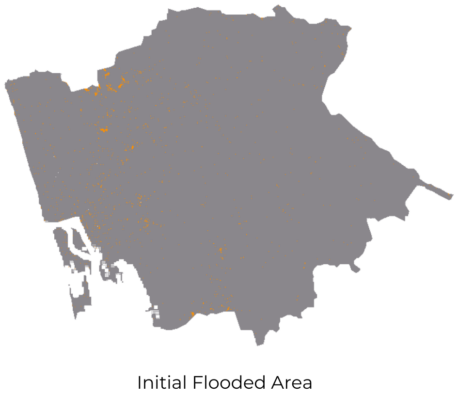
Flooded Area
var admin2 = ee.FeatureCollection("FAO/GAUL_SIMPLIFIED_500m/2015/level2");

var beforeStart = '2018-07-15';
var beforeEnd = '2018-08-10';
var afterStart = '2018-08-10';
var afterEnd = '2018-08-23';

var ernakulam = admin2.filter(ee.Filter.eq('ADM2_NAME', 'Ernakulam'));
var geometry = ernakulam.geometry();
Map.addLayer(geometry, {color: 'grey'}, 'Ernakulam District');

var collection= ee.ImageCollection('COPERNICUS/S1_GRD')
  .filter(ee.Filter.eq('instrumentMode','IW'))
  .filter(ee.Filter.listContains('transmitterReceiverPolarisation', 'VH'))
  .filter(ee.Filter.eq('orbitProperties_pass', 'DESCENDING'))
  .filter(ee.Filter.eq('resolution_meters',10))
  .filter(ee.Filter.bounds(geometry))
  .select('VH');

var beforeCollection = collection
  .filter(ee.Filter.date(beforeStart, beforeEnd));

var afterCollection = collection
  .filter(ee.Filter.date(afterStart, afterEnd));

var before = beforeCollection.mosaic().clip(geometry);
var after = afterCollection.mosaic().clip(geometry);

var beforeFiltered = ee.Image(toDB(RefinedLee(toNatural(before))));
var afterFiltered = ee.Image(toDB(RefinedLee(toNatural(after))));

Map.centerObject(geometry, 10);
Map.addLayer(before, {min:-25,max:0}, 'Before Floods', false);
Map.addLayer(after, {min:-25,max:0}, 'After Floods', false);
Map.addLayer(beforeFiltered, {min:-25,max:0}, 'Before Filtered', false);
Map.addLayer(afterFiltered, {min:-25,max:0}, 'After Filtered', false);

var difference = afterFiltered.divide(beforeFiltered);

// Define a threshold
var diffThreshold = 1.25;
// Initial estimate of flooded pixels
var flooded = difference.gt(diffThreshold).rename('water').selfMask();
Map.addLayer(flooded, {min:0, max:1, palette: ['orange']}, 'Initial Flood Area', false);


//############################
// Speckle Filtering Functions
//############################

// Function to convert from dB
function toNatural(img) {
  return ee.Image(10.0).pow(img.select(0).divide(10.0));
}

//Function to convert to dB
function toDB(img) {
  return ee.Image(img).log10().multiply(10.0);
}

//Apllying a Refined Lee Speckle filter as coded in the SNAP 3.0 S1TBX:

//https://github.com/senbox-org/s1tbx/blob/master/s1tbx-op-sar-processing/src/main/java/org/esa/s1tbx/sar/gpf/filtering/SpeckleFilters/RefinedLee.java
//Adapted by Guido Lemoine

// by Guido Lemoine
function RefinedLee(img) {
  // img must be in natural units, i.e. not in dB!
  // Set up 3x3 kernels
  var weights3 = ee.List.repeat(ee.List.repeat(1,3),3);
  var kernel3 = ee.Kernel.fixed(3,3, weights3, 1, 1, false);

  var mean3 = img.reduceNeighborhood(ee.Reducer.mean(), kernel3);
  var variance3 = img.reduceNeighborhood(ee.Reducer.variance(), kernel3);

  // Use a sample of the 3x3 windows inside a 7x7 windows to determine gradients and directions
  var sample_weights = ee.List([[0,0,0,0,0,0,0], [0,1,0,1,0,1,0],[0,0,0,0,0,0,0], [0,1,0,1,0,1,0], [0,0,0,0,0,0,0], [0,1,0,1,0,1,0],[0,0,0,0,0,0,0]]);

  var sample_kernel = ee.Kernel.fixed(7,7, sample_weights, 3,3, false);

  // Calculate mean and variance for the sampled windows and store as 9 bands
  var sample_mean = mean3.neighborhoodToBands(sample_kernel);
  var sample_var = variance3.neighborhoodToBands(sample_kernel);

  // Determine the 4 gradients for the sampled windows
  var gradients = sample_mean.select(1).subtract(sample_mean.select(7)).abs();
  gradients = gradients.addBands(sample_mean.select(6).subtract(sample_mean.select(2)).abs());
  gradients = gradients.addBands(sample_mean.select(3).subtract(sample_mean.select(5)).abs());
  gradients = gradients.addBands(sample_mean.select(0).subtract(sample_mean.select(8)).abs());

  // And find the maximum gradient amongst gradient bands
  var max_gradient = gradients.reduce(ee.Reducer.max());

  // Create a mask for band pixels that are the maximum gradient
  var gradmask = gradients.eq(max_gradient);

  // duplicate gradmask bands: each gradient represents 2 directions
  gradmask = gradmask.addBands(gradmask);

  // Determine the 8 directions
  var directions = sample_mean.select(1).subtract(sample_mean.select(4)).gt(sample_mean.select(4).subtract(sample_mean.select(7))).multiply(1);
  directions = directions.addBands(sample_mean.select(6).subtract(sample_mean.select(4)).gt(sample_mean.select(4).subtract(sample_mean.select(2))).multiply(2));
  directions = directions.addBands(sample_mean.select(3).subtract(sample_mean.select(4)).gt(sample_mean.select(4).subtract(sample_mean.select(5))).multiply(3));
  directions = directions.addBands(sample_mean.select(0).subtract(sample_mean.select(4)).gt(sample_mean.select(4).subtract(sample_mean.select(8))).multiply(4));
  // The next 4 are the not() of the previous 4
  directions = directions.addBands(directions.select(0).not().multiply(5));
  directions = directions.addBands(directions.select(1).not().multiply(6));
  directions = directions.addBands(directions.select(2).not().multiply(7));
  directions = directions.addBands(directions.select(3).not().multiply(8));

  // Mask all values that are not 1-8
  directions = directions.updateMask(gradmask);

  // "collapse" the stack into a singe band image (due to masking, each pixel has just one value (1-8) in it's directional band, and is otherwise masked)
  directions = directions.reduce(ee.Reducer.sum());

  //var pal = ['ffffff','ff0000','ffff00', '00ff00', '00ffff', '0000ff', 'ff00ff', '000000'];
  //Map.addLayer(directions.reduce(ee.Reducer.sum()), {min:1, max:8, palette: pal}, 'Directions', false);

  var sample_stats = sample_var.divide(sample_mean.multiply(sample_mean));

  // Calculate localNoiseVariance
  var sigmaV = sample_stats.toArray().arraySort().arraySlice(0,0,5).arrayReduce(ee.Reducer.mean(), [0]);

  // Set up the 7*7 kernels for directional statistics
  var rect_weights = ee.List.repeat(ee.List.repeat(0,7),3).cat(ee.List.repeat(ee.List.repeat(1,7),4));

  var diag_weights = ee.List([[1,0,0,0,0,0,0], [1,1,0,0,0,0,0], [1,1,1,0,0,0,0],
    [1,1,1,1,0,0,0], [1,1,1,1,1,0,0], [1,1,1,1,1,1,0], [1,1,1,1,1,1,1]]);

  var rect_kernel = ee.Kernel.fixed(7,7, rect_weights, 3, 3, false);
  var diag_kernel = ee.Kernel.fixed(7,7, diag_weights, 3, 3, false);

  // Create stacks for mean and variance using the original kernels. Mask with relevant direction.
  var dir_mean = img.reduceNeighborhood(ee.Reducer.mean(), rect_kernel).updateMask(directions.eq(1));
  var dir_var = img.reduceNeighborhood(ee.Reducer.variance(), rect_kernel).updateMask(directions.eq(1));

  dir_mean = dir_mean.addBands(img.reduceNeighborhood(ee.Reducer.mean(), diag_kernel).updateMask(directions.eq(2)));
  dir_var = dir_var.addBands(img.reduceNeighborhood(ee.Reducer.variance(), diag_kernel).updateMask(directions.eq(2)));

  // and add the bands for rotated kernels
  for (var i=1; i<4; i++) {
    dir_mean = dir_mean.addBands(img.reduceNeighborhood(ee.Reducer.mean(), rect_kernel.rotate(i)).updateMask(directions.eq(2*i+1)));
    dir_var = dir_var.addBands(img.reduceNeighborhood(ee.Reducer.variance(), rect_kernel.rotate(i)).updateMask(directions.eq(2*i+1)));
    dir_mean = dir_mean.addBands(img.reduceNeighborhood(ee.Reducer.mean(), diag_kernel.rotate(i)).updateMask(directions.eq(2*i+2)));
    dir_var = dir_var.addBands(img.reduceNeighborhood(ee.Reducer.variance(), diag_kernel.rotate(i)).updateMask(directions.eq(2*i+2)));
  }

  // "collapse" the stack into a single band image (due to masking, each pixel has just one value in it's directional band, and is otherwise masked)
  dir_mean = dir_mean.reduce(ee.Reducer.sum());
  dir_var = dir_var.reduce(ee.Reducer.sum());

  // A finally generate the filtered value
  var varX = dir_var.subtract(dir_mean.multiply(dir_mean).multiply(sigmaV)).divide(sigmaV.add(1.0));

  var b = varX.divide(dir_var);

  var result = dir_mean.add(b.multiply(img.subtract(dir_mean)));
  return(result.arrayFlatten([['sum']]));
}
Exercise
This exercise script is adopted from UN-SPIDER’s recommended approach to computing the flooded region.
Compute the difference image by finding the difference between the after and before images. Use a threshold of -3 (arbitrary value) to identify the initial flooded regions. Click Try in Code Editor to view the complete script.
// There is an alternate way to detect change
// Since the S1_GRD collection has log-scaled DB values, subtract is more appropriate
// If you use subtract(), the threshold value also changes.

// Calculate afterFiltered - beforeFiltered
// Create a flood imagge using a threshold of -3
// Display the results with a 'purple' palette
05. Apply Masks
The Initial flooded map shows all the areas where the possibility of water is logged. But this contains both noise and permanent water. We can mask out the other pixels based on our need to get the exact flooded area. In this exercise, we will mask
Permanent water.
High degree slope area.
Isolated pixels.
The permanent water is detected using the GSW water dataset.
The pixel with a seasonality band greater
than 5 is considered permanent water for this computation. Based on the
ground information, this value can be changed. Using the
updateMask function, we can mask out all the permanent
water pixels.
The slope mask is created using the hydroSheds DEM dataset.
The terrain slope can be calculated from the DEM using
ee.Algorithms.Terrain. The areas with a slope greater than
5 degrees are selected and masked out. Mostly the water detected in this
area is due to noise in the imagery.
The isolated pixel mask is done to reduce the noise. A
single pixel detected as flood in the middle of nowhere must probably be
a noise. Hence, all the pixels with less than 8 connected neighbors can
be considered noise and masked out. To identify the connected pixels, we
can use the connectedPixelCount function to check the
connectedness for a pixel in all possible directions. This function will
return an image where each pixel has the number of connected pixel
counts of the image passed to it. Then, using the boolean function
gt(), select all the connected pixel count greater than
8.
After applying all the filters to the initial flooded area image, the remaining pixels can be considered an original flooded region.
Open in Code Editor ↗Although the computation for the mask is done between images with different resolutions, GEE will convert all the images to the images added in map canvas or resolution mentioned during export. In our case, all the images will be resampled and projected to Sentinel 1 GRD projection.
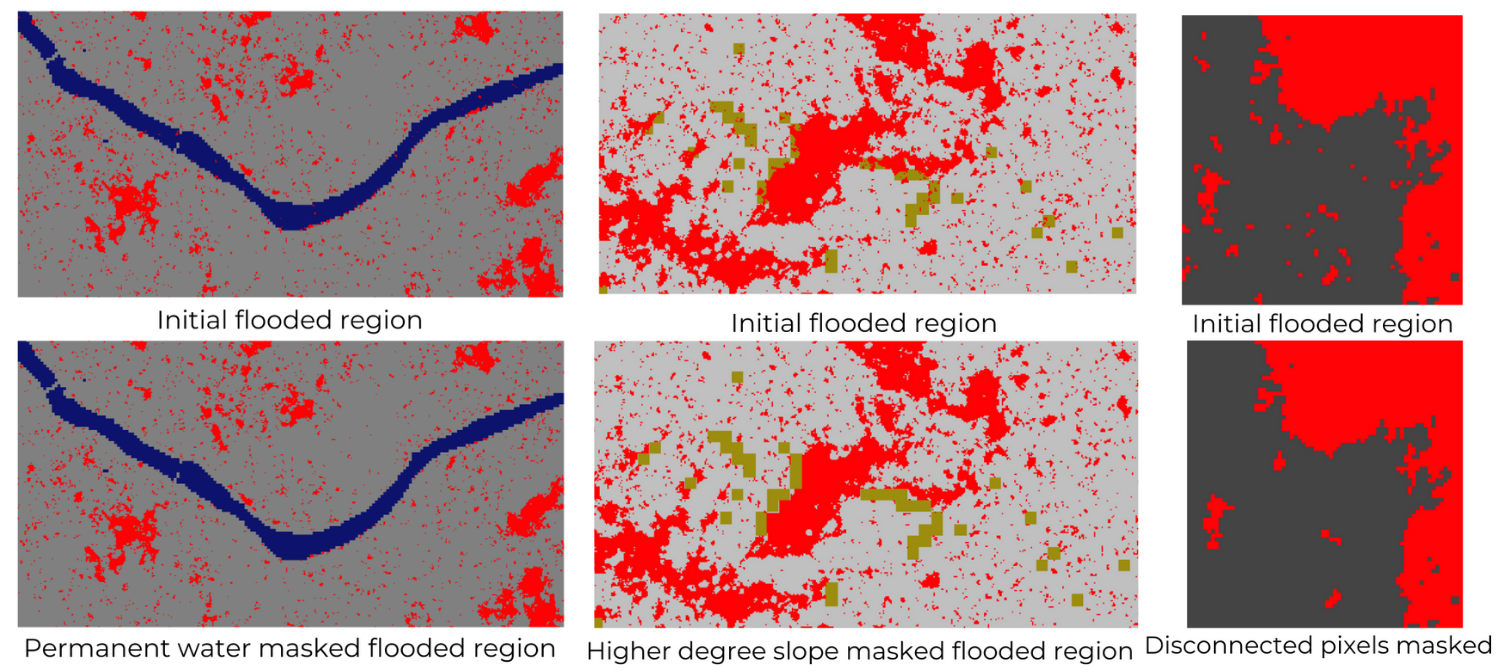
Flood mask
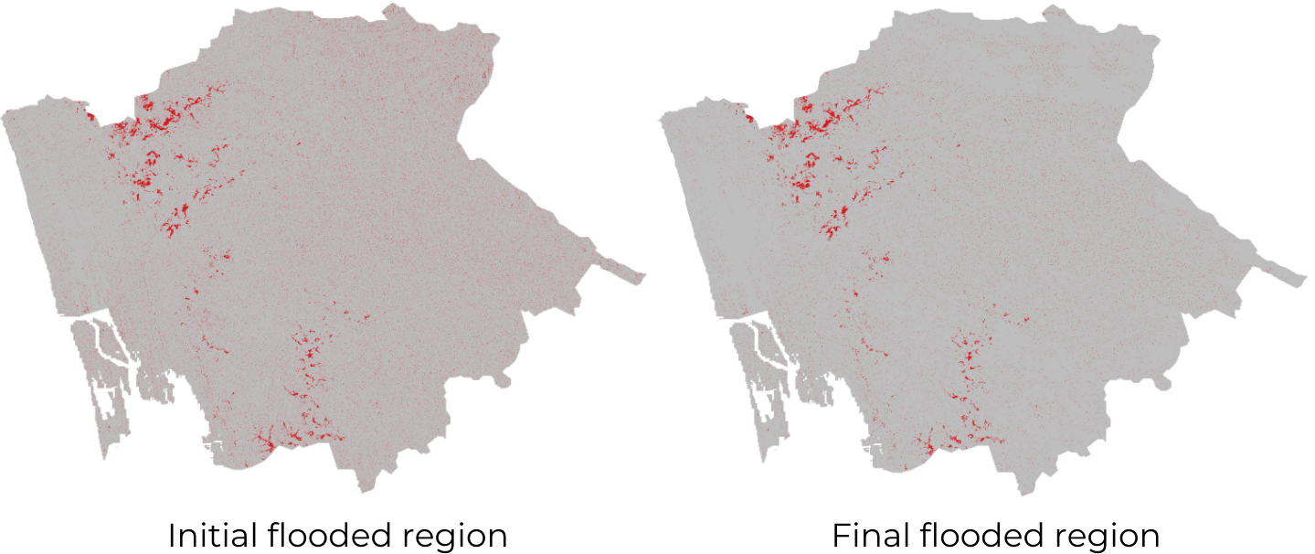
Flooded region
var admin2 = ee.FeatureCollection('FAO/GAUL_SIMPLIFIED_500m/2015/level2');
var hydrosheds = ee.Image('WWF/HydroSHEDS/03VFDEM');
var gsw = ee.Image('JRC/GSW1_4/GlobalSurfaceWater');

var beforeStart = '2018-07-15';
var beforeEnd = '2018-08-10';
var afterStart = '2018-08-10';
var afterEnd = '2018-08-23';

var ernakulam = admin2.filter(ee.Filter.eq('ADM2_NAME', 'Ernakulam'));
var geometry = ernakulam.geometry();
Map.addLayer(geometry, {color: 'grey'}, 'Ernakulam District');

var collection= ee.ImageCollection('COPERNICUS/S1_GRD')
  .filter(ee.Filter.eq('instrumentMode','IW'))
  .filter(ee.Filter.listContains('transmitterReceiverPolarisation', 'VH'))
  .filter(ee.Filter.eq('orbitProperties_pass', 'DESCENDING'))
  .filter(ee.Filter.eq('resolution_meters',10))
  .filter(ee.Filter.bounds(geometry))
  .select('VH');

var beforeCollection = collection
  .filter(ee.Filter.date(beforeStart, beforeEnd));

var afterCollection = collection
  .filter(ee.Filter.date(afterStart, afterEnd));

var before = beforeCollection.mosaic().clip(geometry);
var after = afterCollection.mosaic().clip(geometry);

var beforeFiltered = ee.Image(toDB(RefinedLee(toNatural(before))));
var afterFiltered = ee.Image(toDB(RefinedLee(toNatural(after))));

var difference = afterFiltered.divide(beforeFiltered);

// Define a threshold
var diffThreshold = 1.25;
// Initial estimate of flooded pixels
var flooded = difference.gt(diffThreshold).rename('water').selfMask();

Map.centerObject(geometry, 10);
Map.addLayer(before, {min:-25,max:0}, 'Before Floods', false);
Map.addLayer(after, {min:-25,max:0}, 'After Floods', false);
Map.addLayer(beforeFiltered, {min:-25,max:0}, 'Before Filtered', false);
Map.addLayer(afterFiltered, {min:-25,max:0}, 'After Filtered', false);
Map.addLayer(flooded, {min:0, max:1, palette: ['orange']}, 'Initial Flood Area', false);


// Mask out area with permanent/semi-permanent water
var permanentWater = gsw.select('seasonality').gte(5).clip(geometry);
Map.addLayer(permanentWater.selfMask(),
  {min:0, max:1, palette: ['blue']}, 'Permanent Water', false);

// GSW data is masked in non-water areas. Set it to 0 using unmask()
// Invert the image to set all non-permanent regions to 1
var permanentWaterMask = permanentWater.unmask(0).not();

var flooded = flooded.updateMask(permanentWaterMask);
// Mask out areas with more than 5 percent slope using the HydroSHEDS DEM
var slopeThreshold = 5;
var terrain = ee.Algorithms.Terrain(hydrosheds);
var slope = terrain.select('slope');
var steepAreas = slope.gt(slopeThreshold);
var slopeMask = steepAreas.not();
Map.addLayer(steepAreas.selfMask(),
  {min:0, max:1, palette: ['cyan']}, 'Steep Areas', false);

var flooded = flooded.updateMask(slopeMask);

// Remove isolated pixels
// connectedPixelCount is Zoom dependent, so visual result will vary
var connectedPixelThreshold = 8;
var connections = flooded.connectedPixelCount(25);
var disconnectedAreas = connections.lt(connectedPixelThreshold);
var disconnectedAreasMask = disconnectedAreas.not();
Map.addLayer(disconnectedAreas.selfMask(),
  {min:0, max:1, palette: ['yellow']}, 'Disconnected Areas', false);

var flooded = flooded.updateMask(disconnectedAreasMask);

Map.addLayer(flooded, {min:0, max:1, palette: ['red']}, 'Flooded Areas');


//############################
// Speckle Filtering Functions
//############################

// Function to convert from dB
function toNatural(img) {
  return ee.Image(10.0).pow(img.select(0).divide(10.0));
}

//Function to convert to dB
function toDB(img) {
  return ee.Image(img).log10().multiply(10.0);
}

//Apllying a Refined Lee Speckle filter as coded in the SNAP 3.0 S1TBX:

//https://github.com/senbox-org/s1tbx/blob/master/s1tbx-op-sar-processing/src/main/java/org/esa/s1tbx/sar/gpf/filtering/SpeckleFilters/RefinedLee.java
//Adapted by Guido Lemoine

// by Guido Lemoine
function RefinedLee(img) {
  // img must be in natural units, i.e. not in dB!
  // Set up 3x3 kernels
  var weights3 = ee.List.repeat(ee.List.repeat(1,3),3);
  var kernel3 = ee.Kernel.fixed(3,3, weights3, 1, 1, false);

  var mean3 = img.reduceNeighborhood(ee.Reducer.mean(), kernel3);
  var variance3 = img.reduceNeighborhood(ee.Reducer.variance(), kernel3);

  // Use a sample of the 3x3 windows inside a 7x7 windows to determine gradients and directions
  var sample_weights = ee.List([[0,0,0,0,0,0,0], [0,1,0,1,0,1,0],[0,0,0,0,0,0,0], [0,1,0,1,0,1,0], [0,0,0,0,0,0,0], [0,1,0,1,0,1,0],[0,0,0,0,0,0,0]]);

  var sample_kernel = ee.Kernel.fixed(7,7, sample_weights, 3,3, false);

  // Calculate mean and variance for the sampled windows and store as 9 bands
  var sample_mean = mean3.neighborhoodToBands(sample_kernel);
  var sample_var = variance3.neighborhoodToBands(sample_kernel);

  // Determine the 4 gradients for the sampled windows
  var gradients = sample_mean.select(1).subtract(sample_mean.select(7)).abs();
  gradients = gradients.addBands(sample_mean.select(6).subtract(sample_mean.select(2)).abs());
  gradients = gradients.addBands(sample_mean.select(3).subtract(sample_mean.select(5)).abs());
  gradients = gradients.addBands(sample_mean.select(0).subtract(sample_mean.select(8)).abs());

  // And find the maximum gradient amongst gradient bands
  var max_gradient = gradients.reduce(ee.Reducer.max());

  // Create a mask for band pixels that are the maximum gradient
  var gradmask = gradients.eq(max_gradient);

  // duplicate gradmask bands: each gradient represents 2 directions
  gradmask = gradmask.addBands(gradmask);

  // Determine the 8 directions
  var directions = sample_mean.select(1).subtract(sample_mean.select(4)).gt(sample_mean.select(4).subtract(sample_mean.select(7))).multiply(1);
  directions = directions.addBands(sample_mean.select(6).subtract(sample_mean.select(4)).gt(sample_mean.select(4).subtract(sample_mean.select(2))).multiply(2));
  directions = directions.addBands(sample_mean.select(3).subtract(sample_mean.select(4)).gt(sample_mean.select(4).subtract(sample_mean.select(5))).multiply(3));
  directions = directions.addBands(sample_mean.select(0).subtract(sample_mean.select(4)).gt(sample_mean.select(4).subtract(sample_mean.select(8))).multiply(4));
  // The next 4 are the not() of the previous 4
  directions = directions.addBands(directions.select(0).not().multiply(5));
  directions = directions.addBands(directions.select(1).not().multiply(6));
  directions = directions.addBands(directions.select(2).not().multiply(7));
  directions = directions.addBands(directions.select(3).not().multiply(8));

  // Mask all values that are not 1-8
  directions = directions.updateMask(gradmask);

  // "collapse" the stack into a singe band image (due to masking, each pixel has just one value (1-8) in it's directional band, and is otherwise masked)
  directions = directions.reduce(ee.Reducer.sum());

  //var pal = ['ffffff','ff0000','ffff00', '00ff00', '00ffff', '0000ff', 'ff00ff', '000000'];
  //Map.addLayer(directions.reduce(ee.Reducer.sum()), {min:1, max:8, palette: pal}, 'Directions', false);

  var sample_stats = sample_var.divide(sample_mean.multiply(sample_mean));

  // Calculate localNoiseVariance
  var sigmaV = sample_stats.toArray().arraySort().arraySlice(0,0,5).arrayReduce(ee.Reducer.mean(), [0]);

  // Set up the 7*7 kernels for directional statistics
  var rect_weights = ee.List.repeat(ee.List.repeat(0,7),3).cat(ee.List.repeat(ee.List.repeat(1,7),4));

  var diag_weights = ee.List([[1,0,0,0,0,0,0], [1,1,0,0,0,0,0], [1,1,1,0,0,0,0],
    [1,1,1,1,0,0,0], [1,1,1,1,1,0,0], [1,1,1,1,1,1,0], [1,1,1,1,1,1,1]]);

  var rect_kernel = ee.Kernel.fixed(7,7, rect_weights, 3, 3, false);
  var diag_kernel = ee.Kernel.fixed(7,7, diag_weights, 3, 3, false);

  // Create stacks for mean and variance using the original kernels. Mask with relevant direction.
  var dir_mean = img.reduceNeighborhood(ee.Reducer.mean(), rect_kernel).updateMask(directions.eq(1));
  var dir_var = img.reduceNeighborhood(ee.Reducer.variance(), rect_kernel).updateMask(directions.eq(1));

  dir_mean = dir_mean.addBands(img.reduceNeighborhood(ee.Reducer.mean(), diag_kernel).updateMask(directions.eq(2)));
  dir_var = dir_var.addBands(img.reduceNeighborhood(ee.Reducer.variance(), diag_kernel).updateMask(directions.eq(2)));

  // and add the bands for rotated kernels
  for (var i=1; i<4; i++) {
    dir_mean = dir_mean.addBands(img.reduceNeighborhood(ee.Reducer.mean(), rect_kernel.rotate(i)).updateMask(directions.eq(2*i+1)));
    dir_var = dir_var.addBands(img.reduceNeighborhood(ee.Reducer.variance(), rect_kernel.rotate(i)).updateMask(directions.eq(2*i+1)));
    dir_mean = dir_mean.addBands(img.reduceNeighborhood(ee.Reducer.mean(), diag_kernel.rotate(i)).updateMask(directions.eq(2*i+2)));
    dir_var = dir_var.addBands(img.reduceNeighborhood(ee.Reducer.variance(), diag_kernel.rotate(i)).updateMask(directions.eq(2*i+2)));
  }

  // "collapse" the stack into a single band image (due to masking, each pixel has just one value in it's directional band, and is otherwise masked)
  dir_mean = dir_mean.reduce(ee.Reducer.sum());
  dir_var = dir_var.reduce(ee.Reducer.sum());

  // A finally generate the filtered value
  var varX = dir_var.subtract(dir_mean.multiply(dir_mean).multiply(sigmaV)).divide(sigmaV.add(1.0));

  var b = varX.divide(dir_var);

  var result = dir_mean.add(b.multiply(img.subtract(dir_mean)));
  return(result.arrayFlatten([['sum']]));
}
Exercise
We just learned to mask permanent water using the GSW water dataset. Now mask the cropland pixels extracted from the ESA worldview dataset and add the layer to canvas.
var admin2 = ee.FeatureCollection('FAO/GAUL_SIMPLIFIED_500m/2015/level2');
var hydrosheds = ee.Image('WWF/HydroSHEDS/03VFDEM');
var gsw = ee.Image('JRC/GSW1_3/GlobalSurfaceWater');

var beforeStart = '2018-07-15';
var beforeEnd = '2018-08-10';
var afterStart = '2018-08-10';
var afterEnd = '2018-08-23';

var ernakulam = admin2.filter(ee.Filter.eq('ADM2_NAME', 'Ernakulam'));
var geometry = ernakulam.geometry();
Map.addLayer(geometry, {color: 'grey'}, 'Ernakulam District');

var collection= ee.ImageCollection('COPERNICUS/S1_GRD')
  .filter(ee.Filter.eq('instrumentMode','IW'))
  .filter(ee.Filter.listContains('transmitterReceiverPolarisation', 'VH'))
  .filter(ee.Filter.eq('orbitProperties_pass', 'DESCENDING'))
  .filter(ee.Filter.eq('resolution_meters',10))
  .filter(ee.Filter.bounds(geometry))
  .select('VH');

var beforeCollection = collection
  .filter(ee.Filter.date(beforeStart, beforeEnd));

var afterCollection = collection
  .filter(ee.Filter.date(afterStart, afterEnd));

var before = beforeCollection.mosaic().clip(geometry);
var after = afterCollection.mosaic().clip(geometry);

var beforeFiltered = ee.Image(toDB(RefinedLee(toNatural(before))));
var afterFiltered = ee.Image(toDB(RefinedLee(toNatural(after))));

var difference = afterFiltered.divide(beforeFiltered);

// Define a threshold
var diffThreshold = 1.25;
// Initial estimate of flooded pixels
var flooded = difference.gt(diffThreshold).rename('water').selfMask();

//Map.centerObject(geometry, 10)
Map.addLayer(before, {min:-25,max:0}, 'Before Floods', false);
Map.addLayer(after, {min:-25,max:0}, 'After Floods', false);
Map.addLayer(beforeFiltered, {min:-25,max:0}, 'Before Filtered', false);
Map.addLayer(afterFiltered, {min:-25,max:0}, 'After Filtered', false);
Map.addLayer(flooded, {min:0, max:1, palette: ['orange']}, 'Initial Flood Area', false);


// Mask out area with permanent/semi-permanent water
var permanentWater = gsw.select('seasonality').gte(5).clip(geometry);
Map.addLayer(permanentWater.selfMask(),
  {min:0, max:1, palette: ['blue']}, 'Permanent Water', false);

// GSW data is masked in non-water areas. Set it to 0 using unmask()
// Invert the image to set all non-permanent regions to 1
var permanentWaterMask = permanentWater.unmask(0).not();

var flooded = flooded.updateMask(permanentWaterMask);
// Mask out areas with more than 5 percent slope using the HydroSHEDS DEM
var slopeThreshold = 5;
var terrain = ee.Algorithms.Terrain(hydrosheds);
var slope = terrain.select('slope');
var steepAreas = slope.gt(slopeThreshold);
var slopeMask = steepAreas.not();
Map.addLayer(steepAreas.selfMask(),
  {min:0, max:1, palette: ['cyan']}, 'Steep Areas', false);

var flooded = flooded.updateMask(slopeMask);

// Remove isolated pixels
// connectedPixelCount is Zoom dependent, so visual result will vary
var connectedPixelThreshold = 8;
var connections = flooded.connectedPixelCount(25);
var disconnectedAreas = connections.lt(connectedPixelThreshold);
var disconnectedAreasMask = disconnectedAreas.not();
Map.addLayer(disconnectedAreas.selfMask(),
  {min:0, max:1, palette: ['yellow']}, 'Disconnected Areas', false);

var flooded = flooded.updateMask(disconnectedAreasMask);

Map.addLayer(flooded, {min:0, max:1, palette: ['red']}, 'Flooded Areas');

// Exercise
// Apply a Crop Mask to asses flood damage to crops
// Use the ESA WorldCover data to extract cropland
var dataset = ee.ImageCollection("ESA/WorldCover/v100").first();
var classification = dataset.select('Map').clip(geometry);
var cropland = classification.eq(40);
Map.addLayer(cropland.selfMask(),
  {min:0, max:1, palette: ['white', 'green']}, 'Cropland');

// Mask all non-cropland and display flooded regions
// Display the result on the map.


//############################
// Speckle Filtering Functions
//############################

// Function to convert from dB
function toNatural(img) {
  return ee.Image(10.0).pow(img.select(0).divide(10.0));
}

//Function to convert to dB
function toDB(img) {
  return ee.Image(img).log10().multiply(10.0);
}

//Apllying a Refined Lee Speckle filter as coded in the SNAP 3.0 S1TBX:

//https://github.com/senbox-org/s1tbx/blob/master/s1tbx-op-sar-processing/src/main/java/org/esa/s1tbx/sar/gpf/filtering/SpeckleFilters/RefinedLee.java
//Adapted by Guido Lemoine

// by Guido Lemoine
function RefinedLee(img) {
  // img must be in natural units, i.e. not in dB!
  // Set up 3x3 kernels
  var weights3 = ee.List.repeat(ee.List.repeat(1,3),3);
  var kernel3 = ee.Kernel.fixed(3,3, weights3, 1, 1, false);

  var mean3 = img.reduceNeighborhood(ee.Reducer.mean(), kernel3);
  var variance3 = img.reduceNeighborhood(ee.Reducer.variance(), kernel3);

  // Use a sample of the 3x3 windows inside a 7x7 windows to determine gradients and directions
  var sample_weights = ee.List([[0,0,0,0,0,0,0], [0,1,0,1,0,1,0],[0,0,0,0,0,0,0], [0,1,0,1,0,1,0], [0,0,0,0,0,0,0], [0,1,0,1,0,1,0],[0,0,0,0,0,0,0]]);

  var sample_kernel = ee.Kernel.fixed(7,7, sample_weights, 3,3, false);

  // Calculate mean and variance for the sampled windows and store as 9 bands
  var sample_mean = mean3.neighborhoodToBands(sample_kernel);
  var sample_var = variance3.neighborhoodToBands(sample_kernel);

  // Determine the 4 gradients for the sampled windows
  var gradients = sample_mean.select(1).subtract(sample_mean.select(7)).abs();
  gradients = gradients.addBands(sample_mean.select(6).subtract(sample_mean.select(2)).abs());
  gradients = gradients.addBands(sample_mean.select(3).subtract(sample_mean.select(5)).abs());
  gradients = gradients.addBands(sample_mean.select(0).subtract(sample_mean.select(8)).abs());

  // And find the maximum gradient amongst gradient bands
  var max_gradient = gradients.reduce(ee.Reducer.max());

  // Create a mask for band pixels that are the maximum gradient
  var gradmask = gradients.eq(max_gradient);

  // duplicate gradmask bands: each gradient represents 2 directions
  gradmask = gradmask.addBands(gradmask);

  // Determine the 8 directions
  var directions = sample_mean.select(1).subtract(sample_mean.select(4)).gt(sample_mean.select(4).subtract(sample_mean.select(7))).multiply(1);
  directions = directions.addBands(sample_mean.select(6).subtract(sample_mean.select(4)).gt(sample_mean.select(4).subtract(sample_mean.select(2))).multiply(2));
  directions = directions.addBands(sample_mean.select(3).subtract(sample_mean.select(4)).gt(sample_mean.select(4).subtract(sample_mean.select(5))).multiply(3));
  directions = directions.addBands(sample_mean.select(0).subtract(sample_mean.select(4)).gt(sample_mean.select(4).subtract(sample_mean.select(8))).multiply(4));
  // The next 4 are the not() of the previous 4
  directions = directions.addBands(directions.select(0).not().multiply(5));
  directions = directions.addBands(directions.select(1).not().multiply(6));
  directions = directions.addBands(directions.select(2).not().multiply(7));
  directions = directions.addBands(directions.select(3).not().multiply(8));

  // Mask all values that are not 1-8
  directions = directions.updateMask(gradmask);

  // "collapse" the stack into a singe band image (due to masking, each pixel has just one value (1-8) in it's directional band, and is otherwise masked)
  directions = directions.reduce(ee.Reducer.sum());

  //var pal = ['ffffff','ff0000','ffff00', '00ff00', '00ffff', '0000ff', 'ff00ff', '000000'];
  //Map.addLayer(directions.reduce(ee.Reducer.sum()), {min:1, max:8, palette: pal}, 'Directions', false);

  var sample_stats = sample_var.divide(sample_mean.multiply(sample_mean));

  // Calculate localNoiseVariance
  var sigmaV = sample_stats.toArray().arraySort().arraySlice(0,0,5).arrayReduce(ee.Reducer.mean(), [0]);

  // Set up the 7*7 kernels for directional statistics
  var rect_weights = ee.List.repeat(ee.List.repeat(0,7),3).cat(ee.List.repeat(ee.List.repeat(1,7),4));

  var diag_weights = ee.List([[1,0,0,0,0,0,0], [1,1,0,0,0,0,0], [1,1,1,0,0,0,0],
    [1,1,1,1,0,0,0], [1,1,1,1,1,0,0], [1,1,1,1,1,1,0], [1,1,1,1,1,1,1]]);

  var rect_kernel = ee.Kernel.fixed(7,7, rect_weights, 3, 3, false);
  var diag_kernel = ee.Kernel.fixed(7,7, diag_weights, 3, 3, false);

  // Create stacks for mean and variance using the original kernels. Mask with relevant direction.
  var dir_mean = img.reduceNeighborhood(ee.Reducer.mean(), rect_kernel).updateMask(directions.eq(1));
  var dir_var = img.reduceNeighborhood(ee.Reducer.variance(), rect_kernel).updateMask(directions.eq(1));

  dir_mean = dir_mean.addBands(img.reduceNeighborhood(ee.Reducer.mean(), diag_kernel).updateMask(directions.eq(2)));
  dir_var = dir_var.addBands(img.reduceNeighborhood(ee.Reducer.variance(), diag_kernel).updateMask(directions.eq(2)));

  // and add the bands for rotated kernels
  for (var i=1; i<4; i++) {
    dir_mean = dir_mean.addBands(img.reduceNeighborhood(ee.Reducer.mean(), rect_kernel.rotate(i)).updateMask(directions.eq(2*i+1)));
    dir_var = dir_var.addBands(img.reduceNeighborhood(ee.Reducer.variance(), rect_kernel.rotate(i)).updateMask(directions.eq(2*i+1)));
    dir_mean = dir_mean.addBands(img.reduceNeighborhood(ee.Reducer.mean(), diag_kernel.rotate(i)).updateMask(directions.eq(2*i+2)));
    dir_var = dir_var.addBands(img.reduceNeighborhood(ee.Reducer.variance(), diag_kernel.rotate(i)).updateMask(directions.eq(2*i+2)));
  }

  // "collapse" the stack into a single band image (due to masking, each pixel has just one value in it's directional band, and is otherwise masked)
  dir_mean = dir_mean.reduce(ee.Reducer.sum());
  dir_var = dir_var.reduce(ee.Reducer.sum());

  // A finally generate the filtered value
  var varX = dir_var.subtract(dir_mean.multiply(dir_mean).multiply(sigmaV)).divide(sigmaV.add(1.0));

  var b = varX.divide(dir_var);

  var result = dir_mean.add(b.multiply(img.subtract(dir_mean)));
  return(result.arrayFlatten([['sum']]));
}
06. Calculate Flooded Area
We visually inspected the flooded regions in the previous exercise, now lets us calculate the total flooded area in hectares and compute the percentage of the area flooded. We have already discussed the technique for calculating area in the earth engine.
Open in Code Editor ↗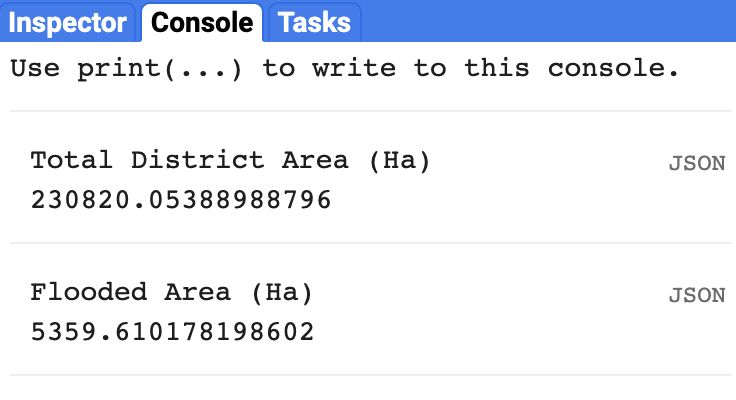
Flooded area
var admin2 = ee.FeatureCollection('FAO/GAUL_SIMPLIFIED_500m/2015/level2');
var hydrosheds = ee.Image('WWF/HydroSHEDS/03VFDEM');
var gsw = ee.Image('JRC/GSW1_3/GlobalSurfaceWater');

var beforeStart = '2018-07-15';
var beforeEnd = '2018-08-10';
var afterStart = '2018-08-10';
var afterEnd = '2018-08-23';

var ernakulam = admin2.filter(ee.Filter.eq('ADM2_NAME', 'Ernakulam'));
var geometry = ernakulam.geometry();
Map.addLayer(geometry, {color: 'grey'}, 'Ernakulam District');

var collection= ee.ImageCollection('COPERNICUS/S1_GRD')
  .filter(ee.Filter.eq('instrumentMode','IW'))
  .filter(ee.Filter.listContains('transmitterReceiverPolarisation', 'VH'))
  .filter(ee.Filter.eq('orbitProperties_pass', 'DESCENDING'))
  .filter(ee.Filter.eq('resolution_meters',10))
  .filter(ee.Filter.bounds(geometry))
  .select('VH');

var beforeCollection = collection
  .filter(ee.Filter.date(beforeStart, beforeEnd));

var afterCollection = collection
  .filter(ee.Filter.date(afterStart, afterEnd));

var before = beforeCollection.mosaic().clip(geometry);
var after = afterCollection.mosaic().clip(geometry);

var beforeFiltered = ee.Image(toDB(RefinedLee(toNatural(before))));
var afterFiltered = ee.Image(toDB(RefinedLee(toNatural(after))));

var difference = afterFiltered.divide(beforeFiltered);

// Define a threshold
var diffThreshold = 1.25;
// Initial estimate of flooded pixels
var flooded = difference.gt(diffThreshold).rename('water').selfMask();

Map.centerObject(geometry, 10);
Map.addLayer(before, {min:-25,max:0}, 'Before Floods', false);
Map.addLayer(after, {min:-25,max:0}, 'After Floods', false);
Map.addLayer(beforeFiltered, {min:-25,max:0}, 'Before Filtered', false);
Map.addLayer(afterFiltered, {min:-25,max:0}, 'After Filtered', false);
Map.addLayer(flooded, {min:0, max:1, palette: ['orange']}, 'Initial Flood Area', false);

// Mask out area with permanent/semi-permanent water
var permanentWater = gsw.select('seasonality').gte(5).clip(geometry);
var permanentWaterMask = permanentWater.unmask(0).not();
var flooded = flooded.updateMask(permanentWaterMask);

// Mask out areas with more than 5 percent slope using the HydroSHEDS DEM
var slopeThreshold = 5;
var terrain = ee.Algorithms.Terrain(hydrosheds);
var slope = terrain.select('slope');
var steepAreas = slope.gt(slopeThreshold);
var slopeMask = steepAreas.not();
var flooded = flooded.updateMask(slopeMask);

// Remove isolated pixels
// connectedPixelCount is Zoom dependent, so visual result will vary
var connectedPixelThreshold = 8;
var connections = flooded.connectedPixelCount(25);
var disconnectedAreas = connections.lt(connectedPixelThreshold);
var disconnectedAreasMask = disconnectedAreas.not();
var flooded = flooded.updateMask(disconnectedAreasMask);

Map.addLayer(flooded, {min:0, max:1, palette: ['red']}, 'Flooded Areas');

// Calculate Affected Area
print('Total District Area (Ha)', geometry.area().divide(10000));

var stats = flooded.multiply(ee.Image.pixelArea()).reduceRegion({
  reducer: ee.Reducer.sum(),
  geometry: geometry,
  scale: 10,
  maxPixels: 1e10,
  tileScale: 16
});
print('Flooded Area (Ha)', ee.Number(stats.get('water')).divide(10000));

//############################
// Speckle Filtering Functions
//############################

// Function to convert from dB
function toNatural(img) {
  return ee.Image(10.0).pow(img.select(0).divide(10.0));
}

//Function to convert to dB
function toDB(img) {
  return ee.Image(img).log10().multiply(10.0);
}

//Apllying a Refined Lee Speckle filter as coded in the SNAP 3.0 S1TBX:

//https://github.com/senbox-org/s1tbx/blob/master/s1tbx-op-sar-processing/src/main/java/org/esa/s1tbx/sar/gpf/filtering/SpeckleFilters/RefinedLee.java
//Adapted by Guido Lemoine

// by Guido Lemoine
function RefinedLee(img) {
  // img must be in natural units, i.e. not in dB!
  // Set up 3x3 kernels
  var weights3 = ee.List.repeat(ee.List.repeat(1,3),3);
  var kernel3 = ee.Kernel.fixed(3,3, weights3, 1, 1, false);

  var mean3 = img.reduceNeighborhood(ee.Reducer.mean(), kernel3);
  var variance3 = img.reduceNeighborhood(ee.Reducer.variance(), kernel3);

  // Use a sample of the 3x3 windows inside a 7x7 windows to determine gradients and directions
  var sample_weights = ee.List([[0,0,0,0,0,0,0], [0,1,0,1,0,1,0],[0,0,0,0,0,0,0], [0,1,0,1,0,1,0], [0,0,0,0,0,0,0], [0,1,0,1,0,1,0],[0,0,0,0,0,0,0]]);

  var sample_kernel = ee.Kernel.fixed(7,7, sample_weights, 3,3, false);

  // Calculate mean and variance for the sampled windows and store as 9 bands
  var sample_mean = mean3.neighborhoodToBands(sample_kernel);
  var sample_var = variance3.neighborhoodToBands(sample_kernel);

  // Determine the 4 gradients for the sampled windows
  var gradients = sample_mean.select(1).subtract(sample_mean.select(7)).abs();
  gradients = gradients.addBands(sample_mean.select(6).subtract(sample_mean.select(2)).abs());
  gradients = gradients.addBands(sample_mean.select(3).subtract(sample_mean.select(5)).abs());
  gradients = gradients.addBands(sample_mean.select(0).subtract(sample_mean.select(8)).abs());

  // And find the maximum gradient amongst gradient bands
  var max_gradient = gradients.reduce(ee.Reducer.max());

  // Create a mask for band pixels that are the maximum gradient
  var gradmask = gradients.eq(max_gradient);

  // duplicate gradmask bands: each gradient represents 2 directions
  gradmask = gradmask.addBands(gradmask);

  // Determine the 8 directions
  var directions = sample_mean.select(1).subtract(sample_mean.select(4)).gt(sample_mean.select(4).subtract(sample_mean.select(7))).multiply(1);
  directions = directions.addBands(sample_mean.select(6).subtract(sample_mean.select(4)).gt(sample_mean.select(4).subtract(sample_mean.select(2))).multiply(2));
  directions = directions.addBands(sample_mean.select(3).subtract(sample_mean.select(4)).gt(sample_mean.select(4).subtract(sample_mean.select(5))).multiply(3));
  directions = directions.addBands(sample_mean.select(0).subtract(sample_mean.select(4)).gt(sample_mean.select(4).subtract(sample_mean.select(8))).multiply(4));
  // The next 4 are the not() of the previous 4
  directions = directions.addBands(directions.select(0).not().multiply(5));
  directions = directions.addBands(directions.select(1).not().multiply(6));
  directions = directions.addBands(directions.select(2).not().multiply(7));
  directions = directions.addBands(directions.select(3).not().multiply(8));

  // Mask all values that are not 1-8
  directions = directions.updateMask(gradmask);

  // "collapse" the stack into a singe band image (due to masking, each pixel has just one value (1-8) in it's directional band, and is otherwise masked)
  directions = directions.reduce(ee.Reducer.sum());

  //var pal = ['ffffff','ff0000','ffff00', '00ff00', '00ffff', '0000ff', 'ff00ff', '000000'];
  //Map.addLayer(directions.reduce(ee.Reducer.sum()), {min:1, max:8, palette: pal}, 'Directions', false);

  var sample_stats = sample_var.divide(sample_mean.multiply(sample_mean));

  // Calculate localNoiseVariance
  var sigmaV = sample_stats.toArray().arraySort().arraySlice(0,0,5).arrayReduce(ee.Reducer.mean(), [0]);

  // Set up the 7*7 kernels for directional statistics
  var rect_weights = ee.List.repeat(ee.List.repeat(0,7),3).cat(ee.List.repeat(ee.List.repeat(1,7),4));

  var diag_weights = ee.List([[1,0,0,0,0,0,0], [1,1,0,0,0,0,0], [1,1,1,0,0,0,0],
    [1,1,1,1,0,0,0], [1,1,1,1,1,0,0], [1,1,1,1,1,1,0], [1,1,1,1,1,1,1]]);

  var rect_kernel = ee.Kernel.fixed(7,7, rect_weights, 3, 3, false);
  var diag_kernel = ee.Kernel.fixed(7,7, diag_weights, 3, 3, false);

  // Create stacks for mean and variance using the original kernels. Mask with relevant direction.
  var dir_mean = img.reduceNeighborhood(ee.Reducer.mean(), rect_kernel).updateMask(directions.eq(1));
  var dir_var = img.reduceNeighborhood(ee.Reducer.variance(), rect_kernel).updateMask(directions.eq(1));

  dir_mean = dir_mean.addBands(img.reduceNeighborhood(ee.Reducer.mean(), diag_kernel).updateMask(directions.eq(2)));
  dir_var = dir_var.addBands(img.reduceNeighborhood(ee.Reducer.variance(), diag_kernel).updateMask(directions.eq(2)));

  // and add the bands for rotated kernels
  for (var i=1; i<4; i++) {
    dir_mean = dir_mean.addBands(img.reduceNeighborhood(ee.Reducer.mean(), rect_kernel.rotate(i)).updateMask(directions.eq(2*i+1)));
    dir_var = dir_var.addBands(img.reduceNeighborhood(ee.Reducer.variance(), rect_kernel.rotate(i)).updateMask(directions.eq(2*i+1)));
    dir_mean = dir_mean.addBands(img.reduceNeighborhood(ee.Reducer.mean(), diag_kernel.rotate(i)).updateMask(directions.eq(2*i+2)));
    dir_var = dir_var.addBands(img.reduceNeighborhood(ee.Reducer.variance(), diag_kernel.rotate(i)).updateMask(directions.eq(2*i+2)));
  }

  // "collapse" the stack into a single band image (due to masking, each pixel has just one value in it's directional band, and is otherwise masked)
  dir_mean = dir_mean.reduce(ee.Reducer.sum());
  dir_var = dir_var.reduce(ee.Reducer.sum());

  // A finally generate the filtered value
  var varX = dir_var.subtract(dir_mean.multiply(dir_mean).multiply(sigmaV)).divide(sigmaV.add(1.0));

  var b = varX.divide(dir_var);

  var result = dir_mean.add(b.multiply(img.subtract(dir_mean)));
  return(result.arrayFlatten([['sum']]));
}
Exercise
Printing the results in the console may timeout for more extensive computations. Convert the flood area numeric value as Feature Collection and export the area as a CSV file. The technique to export numeric values is discussed in Exporting Classified Result.
Module 6: Drought Monitoring
There are many definitions for drought, depending on the context used. Monitoring and calculating the impact of drought in large sales is quite tedious without remote sensing data. In this module, we will learn how to monitor the impact of meteorological drought on natural vegetation by implementing the Vegetation Condition Index (VCI) using the MODIS dataset.

Apart from Hydrological drought, another common drought is the Metrological drought. To track the meteorological drought, rainfall deviation should be calculated. To know more about it, visit Spatial Thought YouTube.
01. Load MODIS NDVI
MODIS Moderate Resolution Imaging Spectroradiometer has many derived products apart from the raw imagery captured every day. There are 2 satellite sensors, Terra and Aqua. The raw images from these satellites are used to produce different data products categorized as Atmospheric products, Land products, Cryosphere products, and Ocean Products. We will use the 16-day composite NDVI data at 250m resolution for this exercise. Also, MODIS follows a unique naming pattern, which helps identify the data.
The product which we use in this exercise is
MOD13Q1.061.
| Name | Meaning |
|---|---|
| MOD | Terra sensor |
| 13Q1 | Vegetation Index at 250m |
| 061 | Version number (use the latest version available at the time of computation) |
Load the Terra Vegetation Indices at 250m resolution and
filter the collection from 2010 to 2020. Each image
has 12 bands, in which NDVI and EVI are the
two vegetation indices bands, other bands contain additional information
about the data at pixel level. NDVI is used to monitor vegetation, but
for very thick vegetation like dense forest, NDVI value will saturate,
and no helpful information can be derived. EVI is used to track and
monitor thick vegetation cover.
var modis = ee.ImageCollection("MODIS/061/MOD13Q1");

var startYear = 2010;
var endYear = 2020;
var startDate = ee.Date.fromYMD(startYear, 1, 1);
var endDate = ee.Date.fromYMD(endYear + 1, 1, 1);
var filtered = modis
  .filter(ee.Filter.date(startDate, endDate));

var modisNDVI = filtered.select('NDVI');

print(modisNDVI);
Exercise
Add the first image to the map be visualizing it using a suitable color palette.
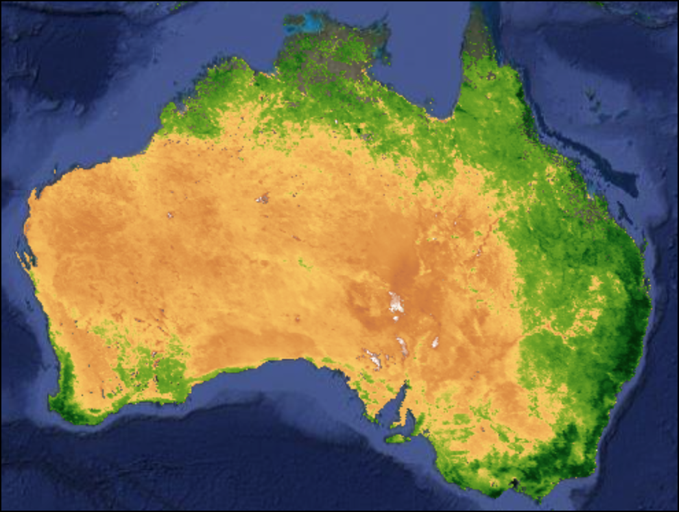
Visualized MODIS NDVI Image over Australia
var modis = ee.ImageCollection("MODIS/061/MOD13Q1");

var startYear = 2010;
var endYear = 2020;
var startDate = ee.Date.fromYMD(startYear, 1, 1);
var endDate = ee.Date.fromYMD(endYear + 1, 1, 1);
var filtered = modis
  .filter(ee.Filter.date(startDate, endDate));

var modisNDVI = filtered.select('NDVI');

print(modisNDVI);

// Exercise

// Extract 1 image from the collection using the .first() function
var image = modisNDVI.first();

// We want to visualize and add the image to the Map
// Add suitable Visualization Parameters to the function below
Map.addLayer(image, {}, 'MODIS NDVI');
02. Apply Cloud Mask
Every image has another band Summary QA, and this band
contains pixel-level information about the quality of data. We want to
keep only the pixels with bit values 0 or 1. We will use the
.leftShift() to create the bitmask for selecting good
quality data.
Bitmasking itself is a complex topic of discussion. Read the blog on Working with QA Bands and Bitmasks to know more about it.
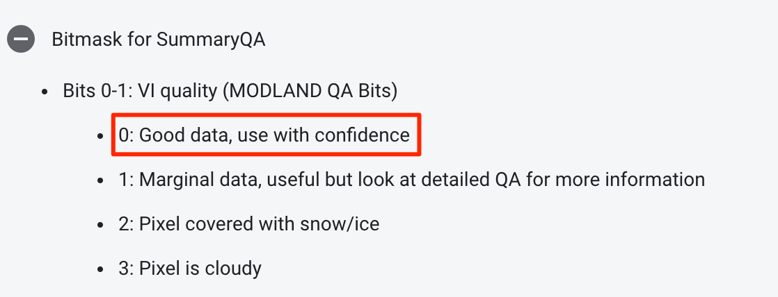
var modis = ee.ImageCollection("MODIS/061/MOD13Q1");

var startYear = 2010;
var endYear = 2020;
var startDate = ee.Date.fromYMD(startYear, 1, 1);
var endDate = ee.Date.fromYMD(endYear + 1, 1, 1);
var filtered = modis
  .filter(ee.Filter.date(startDate, endDate));

// Apply mask to remove low-quality or cloudy pixels
// The data comes with a SummaryQA band
// The values are stored in 2 bits - resulting in 4 possible values
// 0: Good data, use with confidence
// 1: Marginal data, useful but look at detailed QA for more information
// 2: Pixel covered with snow/ice
// 3: Pixel is cloudy
// We want to keep only the pixels with bit values 0 or 1

// Learn about bitmasks
// https://spatialthoughts.com/2021/08/19/qa-bands-bitmasks-gee/
var bitwiseExtract = function(input, fromBit, toBit) {
  var maskSize = ee.Number(1).add(toBit).subtract(fromBit);
  var mask = ee.Number(1).leftShift(maskSize).subtract(1);
  return input.rightShift(fromBit).bitwiseAnd(mask);
};

var maskSnowAndClouds = function(image) {
  var summaryQa = image.select('SummaryQA');
  // Select pixels which are less than or equals to 1 (0 or 1)
  var qaMask = bitwiseExtract(summaryQa, 0, 1).lte(1);
  var maskedImage = image.updateMask(qaMask);
  return maskedImage.copyProperties(image, ['system:index', 'system:time_start']);
};

// Test the function
var image = ee.Image(filtered.first());
var imageMasked = ee.Image(maskSnowAndClouds(image));

Map.addLayer(image, {}, 'MODIS NDVI');
Map.addLayer(imageMasked, {}, 'MODIS NDVI (Masked)'); 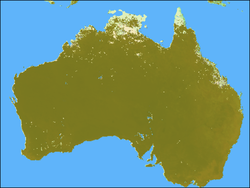
Snow/Cloud Masked MODIS NDVI
Exercise
Use the cloud masking function, pass the filtered collection to get good quality data.
03. Extract and Scale NDVI Band
The NDVI value will be a decimal number ranging between
-2 to 1. But in GEE, each NDVI pixel value
ranges between -20000 to 10000. This is done
to use the storage effectively because an integer number will take less
storage when compared to a floating-point number. Hence, each pixel
value is multiplied by 10,000 and stored as int. Before
using these pixel values for analysis, we can divide each pixel with the
same scale factor as down-scaling to get the original pixel value. We
can find this scale factor information in the data catalog under the
band’s section.
To down-scale each image, we need to pass the image collection into a
function and compute the value for each image. Any computation on the
image will result in a new image with no metadata like
system:timestart of the original image without which timeseries
charting is impossible. So, before returning the image from the
function, we can carry over the required properties using the
.copyProperties() function.
var modis = ee.ImageCollection("MODIS/061/MOD13Q1");

var startYear = 2010;
var endYear = 2020;
var startDate = ee.Date.fromYMD(startYear, 1, 1);
var endDate = ee.Date.fromYMD(endYear + 1, 1, 1);
var filtered = modis
  .filter(ee.Filter.date(startDate, endDate));

// Cloud Masking
var bitwiseExtract = function(input, fromBit, toBit) {
  var maskSize = ee.Number(1).add(toBit).subtract(fromBit);
  var mask = ee.Number(1).leftShift(maskSize).subtract(1);
  return input.rightShift(fromBit).bitwiseAnd(mask);
};

var maskSnowAndClouds = function(image) {
  var summaryQa = image.select('SummaryQA');
  // Select pixels which are less than or equals to 1 (0 or 1)
  var qaMask = bitwiseExtract(summaryQa, 0, 1).lte(1);
  var maskedImage = image.updateMask(qaMask);
  return maskedImage.copyProperties(image, ['system:index', 'system:time_start']);
};

// Apply the function to all images in the collection
var maskedCol = filtered.map(maskSnowAndClouds);

var ndviCol = maskedCol.select('NDVI');

// MODIS NDVI values come as NDVI x 10000 that need to be scaled by 0.0001
var ndviScaled = ndviCol.map(function(image) {
  var scaled = image.divide(10000);
  return scaled.copyProperties(image, ['system:index', 'system:time_start']);
});

print(ndviScaled);
Exercise
Add the scaled image to the map canvas using a suitable visualization parameter. Inspect any pixel and check the NDVI value.
Try in Code Editor ↗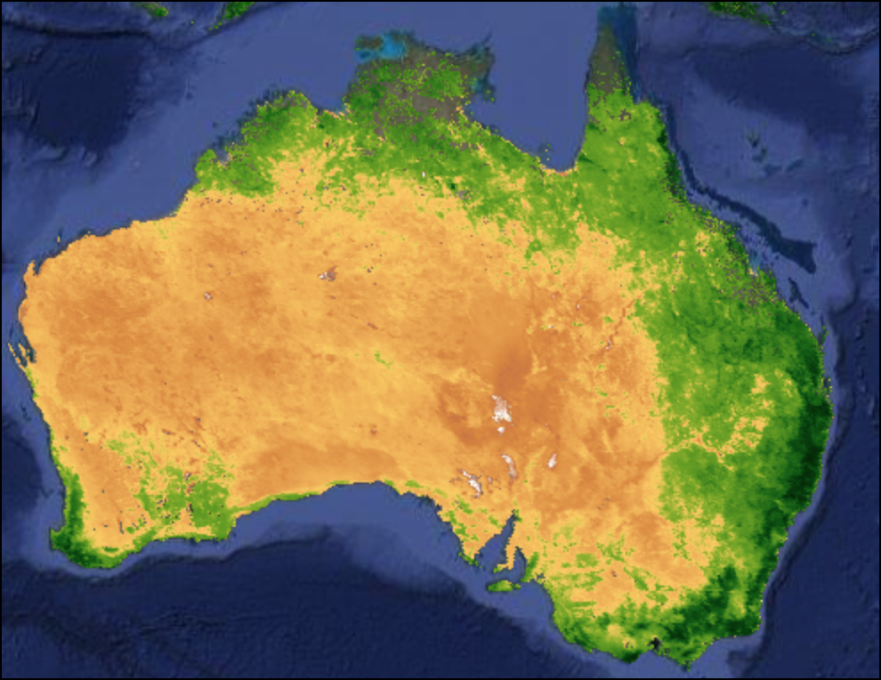
Masked and Scaled MODIS NDVI
04. Create Monthly Images
The MODIS Vegetation Indices is a 16-day composite, and it cannot be
standardized in a calendar unit. So let’s create one image per month by
aggregating all the images in the month as a mean composite. To
filter the collection for with year, month, day level
ee.Filter.calenderRange() function should be use.
We should use a nested map function to map the years first then the
months in the inner map function. The inner months map will return a
Feature Collection, which results in a Feature collection of Feature
Collection when returned by the outer years function. A Feature
collection can contain only Features but not Feature Collection. Hence
we can use the .flatten() algorithm with the outer years
map function to convert Feature collection of Feature
Collection to Feature Collection with List of
Features.
For an 11-year time series, we will create a final output of 132 (11 x 12) images.
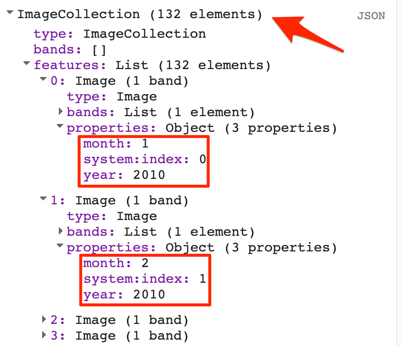
var modis = ee.ImageCollection("MODIS/061/MOD13Q1");

var startYear = 2010;
var endYear = 2020;
var startDate = ee.Date.fromYMD(startYear, 1, 1);
var endDate = ee.Date.fromYMD(endYear + 1, 1, 1);
var filtered = modis
  .filter(ee.Filter.date(startDate, endDate));

// Cloud Masking
var bitwiseExtract = function(input, fromBit, toBit) {
  var maskSize = ee.Number(1).add(toBit).subtract(fromBit);
  var mask = ee.Number(1).leftShift(maskSize).subtract(1);
  return input.rightShift(fromBit).bitwiseAnd(mask);
};

var maskSnowAndClouds = function(image) {
  var summaryQa = image.select('SummaryQA');
  // Select pixels which are less than or equals to 1 (0 or 1)
  var qaMask = bitwiseExtract(summaryQa, 0, 1).lte(1);
  var maskedImage = image.updateMask(qaMask);
  return maskedImage.copyProperties(image, ['system:index', 'system:time_start']);
};

// Apply the function to all images in the collection
var maskedCol = filtered.map(maskSnowAndClouds);

var ndviCol = maskedCol.select('NDVI');

// MODIS NDVI values come as NDVI x 10000 that need to be scaled by 0.0001
var ndviScaled = ndviCol.map(function(image) {
  var scaled = image.divide(10000);
  return scaled.copyProperties(image, ['system:index', 'system:time_start']);
});

print('All Images', ndviScaled);
// Introducting calendarRange()
var mayImages = ndviScaled
  .filter(ee.Filter.calendarRange(5, 5, 'month'));
print('May Images', mayImages);


// Introducting flatten()

var nestedList = ee.List([['a', 'b'], ['c', 'd'], ['e', 'f']]);
print(nestedList);
print(nestedList.flatten());


// Create NDVI composite for every month
var years = ee.List.sequence(startYear,endYear);
var months = ee.List.sequence(1, 12);

// Map over the years and create a monthly average collection
var monthlyImages = years.map(function(year) {
  return months.map(function(month) {
    var filtered = ndviScaled
      .filter(ee.Filter.calendarRange(year, year, 'year'))
      .filter(ee.Filter.calendarRange(month, month, 'month'));
    var monthly = filtered.mean();
    return monthly.set({'month': month, 'year': year});
  });
}).flatten();

// We now have 1 image per month for entire duratioon
print(monthlyImages);

var monthlyCol = ee.ImageCollection.fromImages(monthlyImages);
Exercise
The final output will be a list of images, convert this into an ImageCollection.
05. Calculate Min Max Composites
To compute the VCI, we need to calculate each month’s minimum NDVI
and maximum NDVI values. The min() and max()
reducers are used to compute image collections for the creation of
minimum and maximum NDVI values.
var modis = ee.ImageCollection("MODIS/061/MOD13Q1");

var startYear = 2010;
var endYear = 2020;
var startDate = ee.Date.fromYMD(startYear, 1, 1);
var endDate = ee.Date.fromYMD(endYear + 1, 1, 1);
var filtered = modis
  .filter(ee.Filter.date(startDate, endDate));

// Cloud Masking
var bitwiseExtract = function(input, fromBit, toBit) {
  var maskSize = ee.Number(1).add(toBit).subtract(fromBit);
  var mask = ee.Number(1).leftShift(maskSize).subtract(1);
  return input.rightShift(fromBit).bitwiseAnd(mask);
};

var maskSnowAndClouds = function(image) {
  var summaryQa = image.select('SummaryQA');
  // Select pixels which are less than or equals to 1 (0 or 1)
  var qaMask = bitwiseExtract(summaryQa, 0, 1).lte(1);
  var maskedImage = image.updateMask(qaMask);
  return maskedImage.copyProperties(image, ['system:index', 'system:time_start']);
};

// Apply the function to all images in the collection
var maskedCol = filtered.map(maskSnowAndClouds);

var ndviCol = maskedCol.select('NDVI');

// MODIS NDVI values come as NDVI x 10000 that need to be scaled by 0.0001
var ndviScaled = ndviCol.map(function(image) {
  var scaled = image.divide(10000);
  return scaled.copyProperties(image, ['system:index', 'system:time_start']);
});

// Create NDVI composite for every month
var years = ee.List.sequence(startYear,endYear);
var months = ee.List.sequence(1, 12);

// Map over the years and create a monthly average collection
var monthlyImages = years.map(function(year) {
  return months.map(function(month) {
    var filtered = ndviScaled
      .filter(ee.Filter.calendarRange(year, year, 'year'))
      .filter(ee.Filter.calendarRange(month, month, 'month'));
    var monthly = filtered.mean();
    return monthly.set({'month': month, 'year': year});
  });
}).flatten();

// We now have 1 image per month for entire duratioon
var monthlyCol = ee.ImageCollection.fromImages(monthlyImages);

// We can compute Minimum NDVI for each month across all years
// i.e. Minimum NDVI for all May months in the collection
var monthlyMinImages = months.map(function(month) {
    var filtered = monthlyCol.filter(ee.Filter.eq('month', month));
    var monthlyMin = filtered.min();
    return monthlyMin.set('month', month);
});
var monthlyMin = ee.ImageCollection.fromImages(monthlyMinImages);
print('Monthly Min', monthlyMin);
// We can compute Maximum NDVI for each month across all years
// i.e. Maximum NDVI for all May months in the collection
var monthlyMaxImages = months.map(function(month) {
    var filtered = monthlyCol.filter(ee.Filter.eq('month', month));
    var monthlyMax = filtered.max();
    return monthlyMax.set('month', month);
});
var monthlyMax = ee.ImageCollection.fromImages(monthlyMaxImages);
print('Monthly Max', monthlyMax);
Exercise
Add the min and max NDVI images to map canvas using a suitable visualization parameter for the month of May.
Try in Code Editor ↗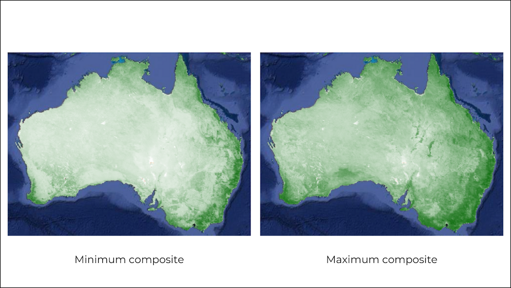
Historic Minimum and Maximum NDVI for the Month of May
06. Calculate VCI
Vegetation Condition Index (VCI) is a drought monitoring index that takes the previous year’s minimum and maximum NDVI values at a particular area and compares it against the current NDVI value to identify if the area is experiencing drought. As recommended by Un-Spider - Drought Monitoring Recommended Practice VCI value of less than 40 % can be considered as drought.
Open in Code Editor ↗
VCI Formula
var modis = ee.ImageCollection("MODIS/061/MOD13Q1");

var startYear = 2010;
var endYear = 2020;
var startDate = ee.Date.fromYMD(startYear, 1, 1);
var endDate = ee.Date.fromYMD(endYear + 1, 1, 1);
var filtered = modis
  .filter(ee.Filter.date(startDate, endDate));

// Cloud Masking
var bitwiseExtract = function(input, fromBit, toBit) {
  var maskSize = ee.Number(1).add(toBit).subtract(fromBit);
  var mask = ee.Number(1).leftShift(maskSize).subtract(1);
  return input.rightShift(fromBit).bitwiseAnd(mask);
};

var maskSnowAndClouds = function(image) {
  var summaryQa = image.select('SummaryQA');
  // Select pixels which are less than or equals to 1 (0 or 1)
  var qaMask = bitwiseExtract(summaryQa, 0, 1).lte(1);
  var maskedImage = image.updateMask(qaMask);
  return maskedImage.copyProperties(image, ['system:index', 'system:time_start']);
};

// Apply the function to all images in the collection
var maskedCol = filtered.map(maskSnowAndClouds);

var ndviCol = maskedCol.select('NDVI');

// MODIS NDVI values come as NDVI x 10000 that need to be scaled by 0.0001
var ndviScaled = ndviCol.map(function(image) {
  var scaled = image.divide(10000);
  return scaled.copyProperties(image, ['system:index', 'system:time_start']);
});

// Create NDVI composite for every month
var years = ee.List.sequence(startYear,endYear);
var months = ee.List.sequence(1, 12);

// Map over the years and create a monthly average collection
var monthlyImages = years.map(function(year) {
  return months.map(function(month) {
    var filtered = ndviScaled
      .filter(ee.Filter.calendarRange(year, year, 'year'))
      .filter(ee.Filter.calendarRange(month, month, 'month'));
    var monthly = filtered.mean();
    return monthly.set({'month': month, 'year': year});
  });
}).flatten();

// We now have 1 image per month for entire duratioon
var monthlyCol = ee.ImageCollection.fromImages(monthlyImages);

// We can compute Minimum NDVI for each month across all years
// i.e. Minimum NDVI for all May months in the collection
var monthlyMinImages = months.map(function(month) {
    var filtered = monthlyCol.filter(ee.Filter.eq('month', month));
    var monthlyMin = filtered.min();
    return monthlyMin.set('month', month);
});
var monthlyMin = ee.ImageCollection.fromImages(monthlyMinImages);
// We can compute Maximum NDVI for each month across all years
// i.e. Maximum NDVI for all May months in the collection
var monthlyMaxImages = months.map(function(month) {
    var filtered = monthlyCol.filter(ee.Filter.eq('month', month));
    var monthlyMax = filtered.max();
    return monthlyMax.set('month', month);
});
var monthlyMax = ee.ImageCollection.fromImages(monthlyMaxImages);

// Calculate VCI for 2020

// We are interested in calculating VCI for a particular month
var currentYear = 2020;
var currentMonth = 5;

var filtered = monthlyCol
  .filter(ee.Filter.eq('year', currentYear))
  .filter(ee.Filter.eq('month', currentMonth));
var currentMonthNdvi = ee.Image(filtered.first());

var minNdvi = ee.Image(monthlyMin.filter(ee.Filter.eq('month', currentMonth)).first());
var maxNdvi = ee.Image(monthlyMax.filter(ee.Filter.eq('month', currentMonth)).first());

// VCI = (NDVI - min) / (max - min)
var image = ee.Image.cat([currentMonthNdvi, minNdvi, maxNdvi]).rename(['ndvi', 'min', 'max']);
var vci = image.expression('100* (ndvi - min) / (max - min)',
    {'ndvi': image.select('ndvi'),
      'min': image.select('min'),
      'max': image.select('max')
    }).rename('vci');


var visParams = {min: 0, max: 1, palette: ['white', 'green']};
var vciPalette = ['#a50026','#d73027','#f46d43','#fdae61',
  '#fee08b','#d9ef8b','#a6d96a','#66bd63','#1a9850','#006837'];
var vciVisParams = {min: 0, max: 100, palette: vciPalette};
Map.addLayer(minNdvi, visParams, 'Minimum May NDVI', false)  ;
Map.addLayer(maxNdvi, visParams, 'Maximum May NDVI', false);
Map.addLayer(currentMonthNdvi, visParams, 'Current May NDVI', false);
Map.addLayer(vci, vciVisParams, 'VCI');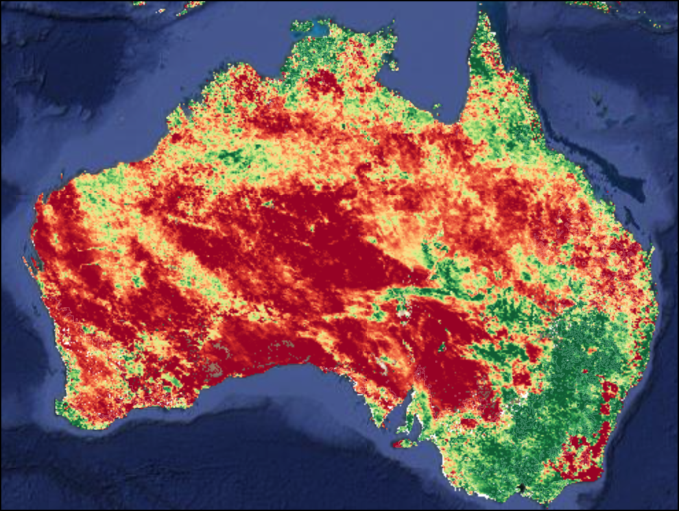
VCI for the Month of May
Exercise
As VCI uses the NDVI index to compute the impact on agriculture. NDVI over non-croplands do not make sense and should be excluded from VCI calculation. Use the Global Food-Support Analysis Data and mask all non-cropland areas.
07. Classify VCI Image
Let us classify the VCI image into 3 categories: Good, Fair, and
Poor. To select a range of values, we can use the boolean
operators. We can use the .where() function to perform
this over an image.
var modis = ee.ImageCollection("MODIS/061/MOD13Q1");

var startYear = 2010;
var endYear = 2020;
var startDate = ee.Date.fromYMD(startYear, 1, 1);
var endDate = ee.Date.fromYMD(endYear + 1, 1, 1);
var filtered = modis
  .filter(ee.Filter.date(startDate, endDate));

// Cloud Masking
var bitwiseExtract = function(input, fromBit, toBit) {
  var maskSize = ee.Number(1).add(toBit).subtract(fromBit);
  var mask = ee.Number(1).leftShift(maskSize).subtract(1);
  return input.rightShift(fromBit).bitwiseAnd(mask);
};

var maskSnowAndClouds = function(image) {
  var summaryQa = image.select('SummaryQA');
  // Select pixels which are less than or equals to 1 (0 or 1)
  var qaMask = bitwiseExtract(summaryQa, 0, 1).lte(1);
  var maskedImage = image.updateMask(qaMask);
  return maskedImage.copyProperties(image, ['system:index', 'system:time_start']);
};

// Apply the function to all images in the collection
var maskedCol = filtered.map(maskSnowAndClouds);

var ndviCol = maskedCol.select('NDVI');

// MODIS NDVI values come as NDVI x 10000 that need to be scaled by 0.0001
var ndviScaled = ndviCol.map(function(image) {
  var scaled = image.divide(10000);
  return scaled.copyProperties(image, ['system:index', 'system:time_start']);
});

// Create NDVI composite for every month
var years = ee.List.sequence(startYear,endYear);
var months = ee.List.sequence(1, 12);

// Map over the years and create a monthly average collection
var monthlyImages = years.map(function(year) {
  return months.map(function(month) {
    var filtered = ndviScaled
      .filter(ee.Filter.calendarRange(year, year, 'year'))
      .filter(ee.Filter.calendarRange(month, month, 'month'));
    var monthly = filtered.mean();
    return monthly.set({'month': month, 'year': year});
  });
}).flatten();

// We now have 1 image per month for entire duratioon
var monthlyCol = ee.ImageCollection.fromImages(monthlyImages);

// We can compute Minimum NDVI for each month across all years
// i.e. Minimum NDVI for all May months in the collection
var monthlyMinImages = months.map(function(month) {
    var filtered = monthlyCol.filter(ee.Filter.eq('month', month));
    var monthlyMin = filtered.min();
    return monthlyMin.set('month', month);
});
var monthlyMin = ee.ImageCollection.fromImages(monthlyMinImages);
// We can compute Maximum NDVI for each month across all years
// i.e. Maximum NDVI for all May months in the collection
var monthlyMaxImages = months.map(function(month) {
    var filtered = monthlyCol.filter(ee.Filter.eq('month', month));
    var monthlyMax = filtered.max();
    return monthlyMax.set('month', month);
});
var monthlyMax = ee.ImageCollection.fromImages(monthlyMaxImages);

// Calculate VCI for 2020

// We are interested in calculating VCI for a particular month
var currentYear = 2020;
var currentMonth = 5;

var filtered = monthlyCol
  .filter(ee.Filter.eq('year', currentYear))
  .filter(ee.Filter.eq('month', currentMonth));
var currentMonthNdvi = ee.Image(filtered.first());

var minNdvi = ee.Image(monthlyMin.filter(ee.Filter.eq('month', currentMonth)).first());
var maxNdvi = ee.Image(monthlyMax.filter(ee.Filter.eq('month', currentMonth)).first());

// VCI = (NDVI - min) / (max - min)
var image = ee.Image.cat([currentMonthNdvi, minNdvi, maxNdvi]).rename(['ndvi', 'min', 'max']);
var vci = image.expression('100* (ndvi - min) / (max - min)',
    {'ndvi': image.select('ndvi'),
      'min': image.select('min'),
      'max': image.select('max')
    }).rename('vci');

var gcep30 = ee.ImageCollection('projects/sat-io/open-datasets/GFSAD/GCEP30');
var cropLand = gcep30.mosaic().eq(2);
var vciMasked = vci.updateMask(cropLand);

// Vegetation Condition Classification

// | VCI    | Condition |
// | 60-100 | Good      |
// | 40-60  | Fair      |
// | 0-40   | Poor      |

// Use .where() function to classify continuous images to
// discrete values
var condition = vciMasked
  .where(vciMasked.lt(40), 1)
  .where(vciMasked.gte(40).and(vciMasked.lt(60)), 2)
  .where(vciMasked.gte(60), 3);

var vciPalette = ['#a50026','#d73027','#f46d43','#fdae61',
  '#fee08b','#d9ef8b','#a6d96a','#66bd63','#1a9850','#006837'];
var vciVisParams = {min: 0, max: 100, palette: vciPalette};
var conditionParams = {min:1, max:3, palette: ['#d7191c','#fdae61','#91cf60']};
Map.addLayer(vciMasked, vciVisParams, 'VCI', false);
Map.addLayer(condition, conditionParams, 'Vegetation Condition');
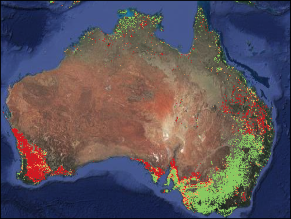
Masked and Classified VCI Image
Exercise
Extract all pixels representing Poor VCI (Value = 1) from the classified VCI image. Apply a Mask and display the regions in ‘red’ color.
Module 7: Earth Engine Apps
The Earth Engine Javascript API includes a ui module
that allows you to build interactive web-mapping apps easily. Earth
Engine also provides free cloud-hosting to host the app that can be
shared with stakeholders. This module will introduce you to GEE Apps by
creating a simple Surface
Water Explorer App.

01. Client vs Server
The User Interface elements in your Code Editor - Map View, Drawing Tools etc. are ‘client-side’ elements. They run in YOUR browser. Image Collections, feature collections, calculations on Earth Engine objects etc. are ‘server-side’ elements. They run in Google’s data center. You cannot mix both these objects. To learn more, visit the Client vs. Server section of the Earth Engine User Guide.
- To convert client-side objects to server-side objects, you can use
the appropriate API function. Server-side functions start with
ee., suchee.Date(),ee.Image()etc. - To convert server-side objects to client-side objects, you can call
.getInfo()on am Earth Engine object. For the Python API, this is the only way to extract information from a server-side object, but the Javascript API provides a better (and preferred) - method for bring server-side objects to client-side using theevaluate()method. This method asynchronously retrieves the value of the object, without blocking the user interface - meaning it will let your code continue to execute while it fetches the value.
// Client vs. Server

// User Interface elements - Map View, Drawing Tools, Buttons, Sliders etc.
// are 'client-side'. They run in YOUR browser

// Image Collections, feature collections, calculations on Earth Engine objects
// etc. are 'server-side'. They run in Google's data center.

// You cannot mix both these objects.

var date = '2020-01-01' // This is client-side
print(typeof(date))

var eedate = ee.Date('2020-01-01').format() // This is server-side
print(typeof(eedate))

// To bring server-side objects to client-side, you can call .getInfo()

// var clientdate = eedate.getInfo()
// print(clientdate)
// print(typeof(clientdate))

// getInfo() blocks the execution of your code till the value is fetched
// If the value takes time to compute, your code editor will freeze
// This is not a good user experience
var s2 = ee.ImageCollection("COPERNICUS/S2_SR_HARMONIZED")
var filtered = s2.filter(ee.Filter.date('2020-01-01', '2020-01-31'))

//var numImages = filtered.size().getInfo()
//print(numImages)

// A better approach is to use evaluate() function
// This is an 'ascynshronous' function - meaning it will let your code
// continue to execute while it fetches the value

// You need to define a 'callback' function which will be called once the
// value has been computed and ready to be used.

var myCallback = function(object) {
  print(object)
}
print('Computing the size of the collection')
var numImages = filtered.size().evaluate(myCallback)
02. Building an App with UI Widgets
Earth Engine comes with a User Interface API that allows you to build an interactive web application powered by Earth Engine. Building a web mapping application typically requires the skills of a full stack developer and are out of reach for most analysts and scientists. But the Earth Engine User Interface API makes this process much more accessible by providing ready-to-use widgets, such as Buttons, Drop-down Menus, Sliders etc. - and free cloud hosting to allow anyone to publish an app with just a few lines of code.
The apps run in your browser, so they need to use
client-side functions. All the user interface functions are
contained in the ui. package - such as
ui.Select(), ui.Button(). You can create those
elements by calling these functions with appropriate parameters. The
main container object is the ui.Panel() which can contain
different types of widgets. Learn more in the Earth Engine
User Interface API section of the Earth Engine User Guide.
The code below shows how to build an app called Surface Water Explorer that allows anyone to pick a district in Karnataka, India then load the JRC Yearly Water Classification History of the district. .
Publishing the App.
We can publish the app to be viewed by anyone regardless of having an account in the earth engine. Click the Apps button in the top left of the script panel and click New apps in the Manage Apps dialog. In the Publish New App dialog, give an app’s name, a public URL will be generated by which we can access the app. Then if you do not have a GCP account, create one and select a project in which you should publish the app. Then with the default settings, click Publish. It will take a few minutes for the earth engine to process your request. After that, your Geo APP will be up and running on the GCP server.
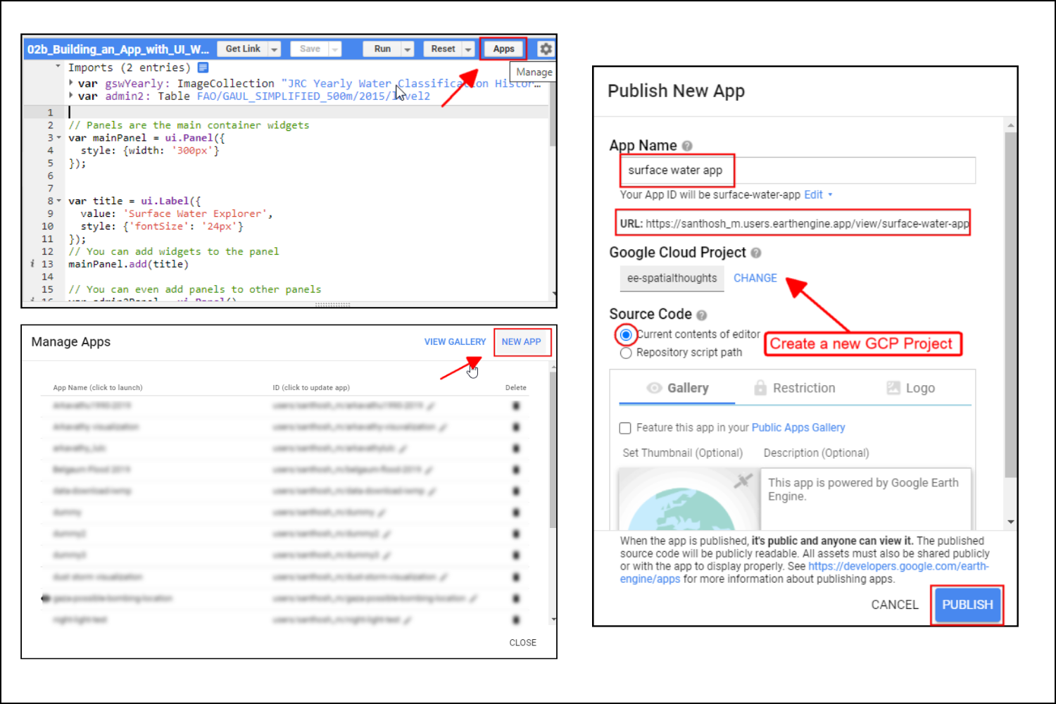
var admin2 = ee.FeatureCollection('FAO/GAUL_SIMPLIFIED_500m/2015/level2');
var gswYearly = ee.ImageCollection('JRC/GSW1_3/YearlyHistory');

// Panels are the main container widgets
var mainPanel = ui.Panel({
  style: {width: '300px'}
});


var title = ui.Label({
  value: 'Surface Water Explorer',
  style: {'fontSize': '24px'}
});
// You can add widgets to the panel
mainPanel.add(title);

// You can even add panels to other panels
var admin2Panel = ui.Panel();
mainPanel.add(admin2Panel);

// Let's add a dropdown with the names of admin2 regions
// We need to get all admin2 names and creat a ui.Select object

var filtered = admin2.filter(ee.Filter.eq('ADM1_NAME', 'Karnataka'));
var admin2Names = filtered.aggregate_array('ADM2_NAME');

// We define a function that will be called when the user selects a value
admin2Names.evaluate(function(names){
  var dropDown = ui.Select({
    placeholder: 'select a region',
    items: names,
    onChange: display
  });
  admin2Panel.add(dropDown);
});

// This function will be called when the user changes the value in the dropdown
var display = function(admin2Name) {
  var selected = ee.Feature(
    filtered.filter(ee.Filter.eq('ADM2_NAME', admin2Name)).first());
  var geometry = selected.geometry();
  Map.clear();
  Map.addLayer(geometry, {color: 'grey'}, admin2Name);
  Map.centerObject(geometry, 10);

  var gswYearFiltered = gswYearly.filter(ee.Filter.eq('year', 2020));
  var gsw2020 = ee.Image(gswYearFiltered.first()).clip(geometry);
  var water2020 = gsw2020.eq(2).or(gsw2020.eq(3)).rename('water').selfMask();

  var visParams = {min:0, max:1, palette: ['white','blue']};
  Map.addLayer(water2020, visParams, '2020 Water');
};

Map.setCenter(76.43, 12.41, 8);
ui.root.add(mainPanel);
Exercise
Create the app for your location.
03. Performing Calculations
We can also perform calculations based on user input, and we can do
this by using the onChange and evaluate()
function. Any UI algorithm that accepts user information will have an
option called onChange, and this will initiate a function if
the user changes the value. We need to perform calculations only after
the data is retrieved for user inputs, and this can be done using the
evaluate function, which works asynchronously without affecting
other computations.
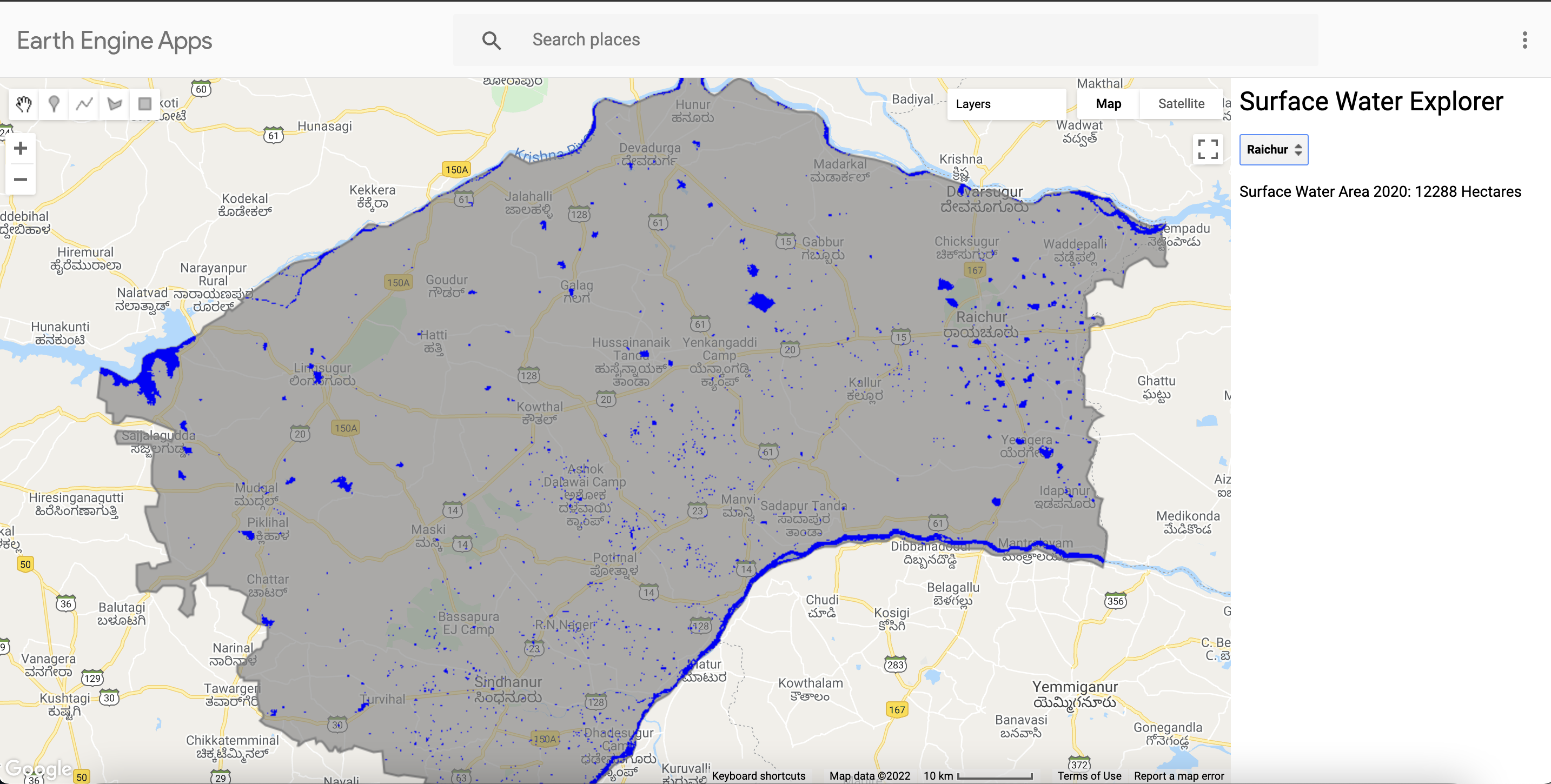
var admin2 = ee.FeatureCollection('FAO/GAUL_SIMPLIFIED_500m/2015/level2');
var gswYearly = ee.ImageCollection('JRC/GSW1_3/YearlyHistory');

// Panels are the main container widgets
var mainPanel = ui.Panel({
  style: {width: '300px'}
});


var title = ui.Label({
  value: 'Surface Water Explorer',
  style: {'fontSize': '24px'}
});
// You can add widgets to the panel
mainPanel.add(title);

// You can even add panels to other panels
var admin2Panel = ui.Panel();
mainPanel.add(admin2Panel);

// Add a panel to display area
var resultPanel = ui.Panel();
var areaLabel = ui.Label();
resultPanel.add(areaLabel);

mainPanel.add(resultPanel);

// This function will be called when the user changes the value in the dropdown
var display = function(admin2Name) {
  areaLabel.setValue('');
  var selected = ee.Feature(
    filtered.filter(ee.Filter.eq('ADM2_NAME', admin2Name)).first());
  var geometry = selected.geometry();
  Map.clear();
  Map.addLayer(geometry, {color: 'grey'}, admin2Name);
  Map.centerObject(geometry, 10);

  var gswYearFiltered = gswYearly.filter(ee.Filter.eq('year', 2020));
  var gsw2020 = ee.Image(gswYearFiltered.first()).clip(geometry);
  var water2020 = gsw2020.eq(2).or(gsw2020.eq(3)).rename('water').selfMask();

  var visParams = {min:0, max:1, palette: ['white','blue']};
  Map.addLayer(water2020, visParams, '2020 Water');

  var area = water2020.multiply(ee.Image.pixelArea()).reduceRegion({
    reducer: ee.Reducer.sum(),
    geometry: geometry,
    scale: 30,
    maxPixels: 1e9
  });

  var waterArea = ee.Number(area.get('water')).divide(10000).round();
  waterArea.evaluate(function(result) {
    var text = 'Surface Water Area 2020: ' + result + ' Hectares';
    areaLabel.setValue(text);
  });
};

// Let's add a dropdown with the names of admin2 regions
// We need to get all admin2 names and creat a ui.Select object

var filtered = admin2.filter(ee.Filter.eq('ADM1_NAME', 'Karnataka'));
var admin2Names = filtered.aggregate_array('ADM2_NAME');

// We define a function that will be called when the user selects a value
admin2Names.evaluate(function(names){
  var dropDown = ui.Select({
    placeholder: 'select a region',
    items: names,
    onChange: display
  });
  admin2Panel.add(dropDown);
});


Map.setCenter(76.43, 12.41, 8);
ui.root.add(mainPanel);
Exercise
Before publishing your app, add your name as Author.
Supplement
Drought Monitoring
Pie Chart Group Statistics
This section has been moved to the Supplement at Pie Chart Group Statistics.
Hydrology
Chart Cumulative Rainfall
This section has been moved to the Supplement at Chart Cumulative Rainfall.
Exporting Precipitation Data
This section has been moved to the Supplement at Exporting Precipitation Data.
GPM Precipitation Time Series
This section has been moved to the Supplement at GPM Precipitation Time Series.
IMD Number of Rainy Days
This section has been moved to the Supplement at IMD Number of Rainy Days.
Surface Water
Detect First Year of Water
This section has been moved to the Supplement at Detect First Year of Water.
Otsu Dynamic Thresholding
This section has been moved to the Supplement at Otsu Dynamic Thresholding.
Smoothing Vectors
This section has been moved to the Supplement at Smoothing Vectors.
Surface Water Explorer Split Panel App
This section has been moved to the Supplement at Surface Water Explorer Split Panel App.
Unsupervised Clustering Advanced
This section has been moved to the Supplement at Unsupervised Clustering Advanced.
SAR
Sentinel-1 ARD Pre-Processing
This section has been moved to the Supplement at Sentinel-1 ARD Pre-Processing.
Time Series Analysis
Mann Kendall Test
This section has been moved to the Supplement at Mann Kendall Test.
Data Credits
Sentinel-2 Level-1C, Level-2A and Sentinel-1 SAR GRD: Contains Copernicus Sentinel data.
TerraClimate: Monthly Climate and Climatic Water Balance for Global Terrestrial Surfaces, University of Idaho: Abatzoglou, J.T., S.Z. Dobrowski, S.A. Parks, K.C. Hegewisch, 2018, Terraclimate, a high-resolution global dataset of monthly climate and climatic water balance from 1958-2015, Scientific Data 5:170191, doi:10.1038/sdata.2017.191
FAO GAUL 500m: Global Administrative Unit Layers 2015, Second-Level Administrative Units: Source of Administrative boundaries: The Global Administrative Unit Layers (GAUL) dataset, implemented by FAO within the CountrySTAT and Agricultural Market Information System (AMIS) projects.
CHIRPS Pentad: Climate Hazards Group InfraRed Precipitation with Station Data (version 2.0 final): Funk, Chris, Pete Peterson, Martin Landsfeld, Diego Pedreros, James Verdin, Shraddhanand Shukla, Gregory Husak, James Rowland, Laura Harrison, Andrew Hoell & Joel Michaelsen. “The climate hazards infrared precipitation with stations—a new environmental record for monitoring extremes”. Scientific Data 2, 150066. doi:10.1038/sdata.2015.66 2015.
MOD13Q1.006 Terra Vegetation Indices 16-Day Global 250m: Didan, K. (2015). MOD13Q1 MODIS/Terra Vegetation Indices 16-Day L3 Global 250m SIN Grid V006 [Data set]. NASA EOSDIS Land Processes DAAC. Accessed 2021-05-06 from https://doi.org/10.5067/MODIS/MOD13Q1.006
License
The course material (text, images, presentation, videos) is licensed under a Creative Commons Attribution 4.0 International License.
The code (scripts, Jupyter notebooks) is licensed under the MIT License. For a copy, see https://opensource.org/licenses/MIT
Kindly give appropriate credit to the original author as below:
Copyright © 2021 Ujaval Gandhi www.spatialthoughts.com
Citing and Referencing
You can cite the course materials as follows
- Gandhi, Ujaval, 2021. Google Earth Engine for Water Resources Management Course. Spatial Thoughts. https://courses.spatialthoughts.com/gee-water-resources-management.html
This course is offered as an instructor-led online class. Visit Spatial Thoughts to know details of upcoming sessions.
If you want to report any issues with this page, please comment below.