Cloud Native Geospatial Workflows with QGIS (Full workshop)
Using QGIS for visualizing and analyzing large cloud-hosted raster and vector datasets.
Ujaval Gandhi
![]()
Introduction
This workshop introduces participants to the modern approach to working with large datasets in QGIS. Modern data formats - such as Cloud-Optimized GeoTIFFs (COG), Cloud-Optimized Point Clouds (COPC), and FlatGeoBuf (FGB) allow datasets to be streamed from cloud storage without having to download entire files. Spatial Temporal Asset Catalog (STAC) provides a standardized way to query cloud-hosted datasets. Combined with QGIS, these technologies allow users to visualize and analyze large datasets which was not possible before.
Installation and Setting up the Environment
Install QGIS
This workshop requires QGIS LTR version 3.44. Please review QGIS-LTR Installation Guide for step-by-step instructions.
Get the Data Package
We have created a data package containing checkpoint projects that will allow you to load the results of each section. You can download the data package from qgis_cloud_native_geospatial.zip. Once downloaded, unzip the contents to a folder on your computer.
1. Cloud Native Geospatial Formats
1.1 Load a Cloud-Optimized GeoTIFF (COG)
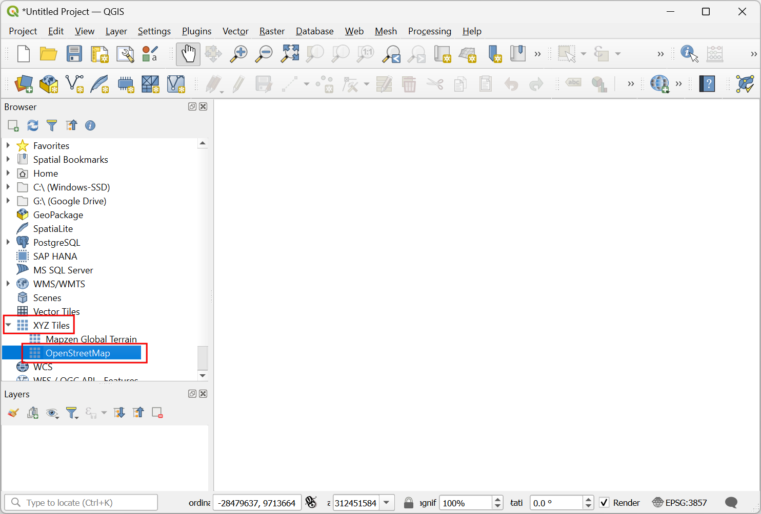
- Open QGIS. We’ll first load a basemap. From the Browser panel, scroll down and locate XYZ Tiles → OpenStreetMap tile layer. Drag and drop it to the main canvas.
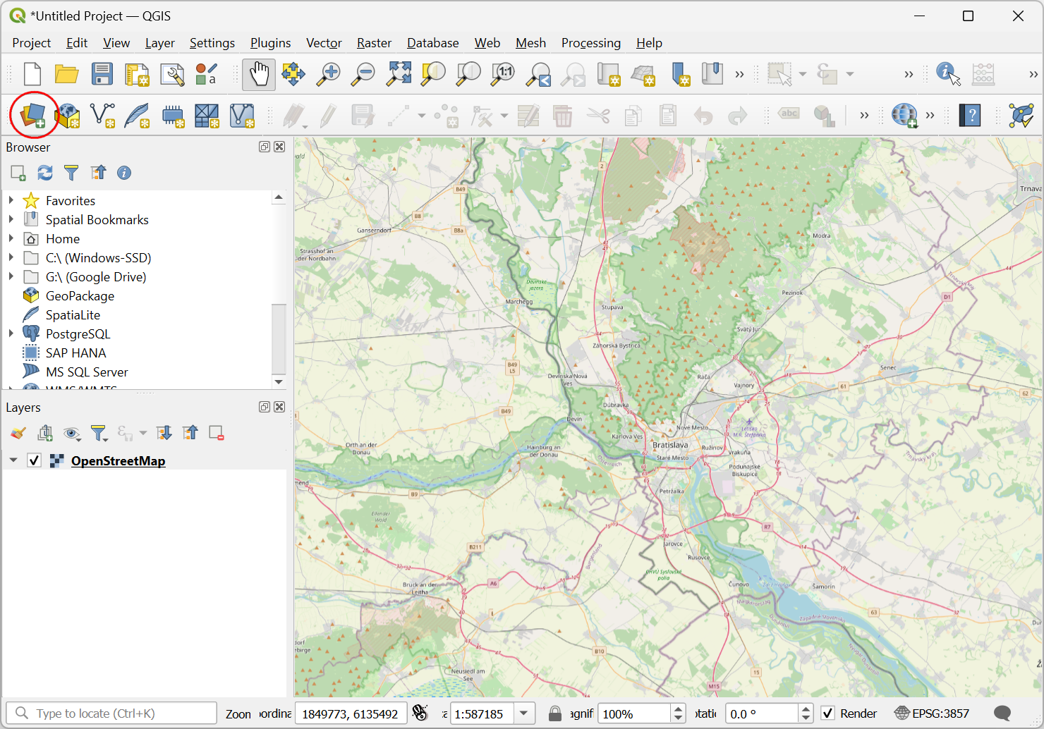
- Once the
OpenStreetMaplayer is loaded, go to your region of interest. Now we will load a 8GB cloud-optimized geotiff file stored on Google Cloud Storage and stream the pixels over this region. Click the Open Data Source Manager button.
- Select the Raster tab. Select
Protocol: HTTP(S), cloud etc.as the Source Type. Enter the following URL as the URI. Click Add.
https://storage.googleapis.com/spatialthoughts-public-data/ntl/viirs/viirs_ntl_2021_global.tif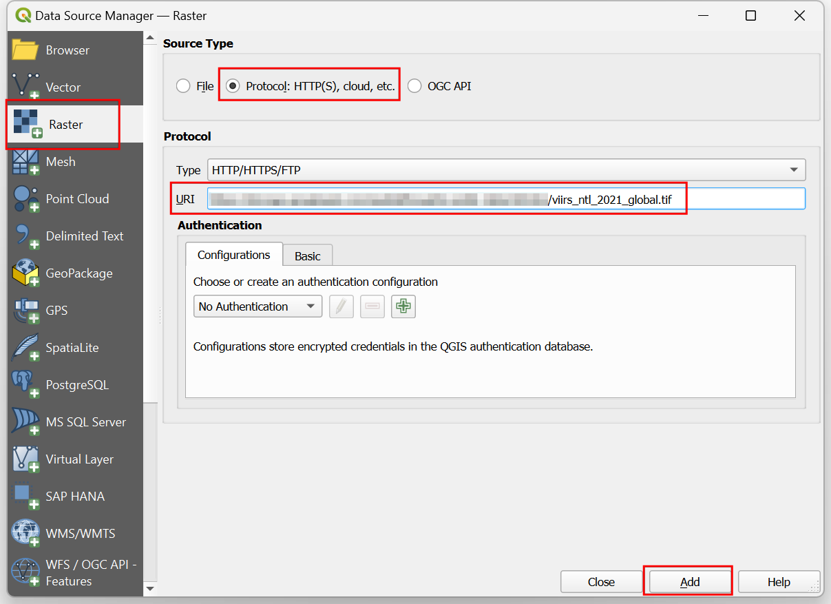
- A new layer
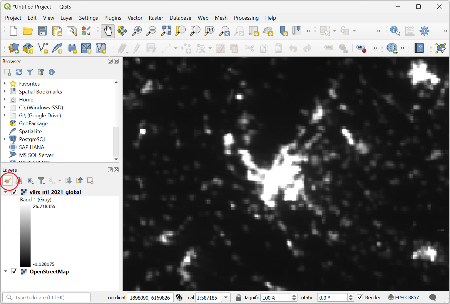
viirs_ntl_2021_globalwill be added to the Layers panel. This is a global layer showing nighttime lights intensity values recorded by the VIIRS instrument. Note that the file loaded instantly and as you zoom in further, higher resolution pixels are fetched dynamically from the file. While this file is located on a remote location, you can use it just as if it was a regular GeoTIFF file. Let’s visualize the layer using a color-ramp. Click the Open Layer Styling Panel button on the Layers panel.
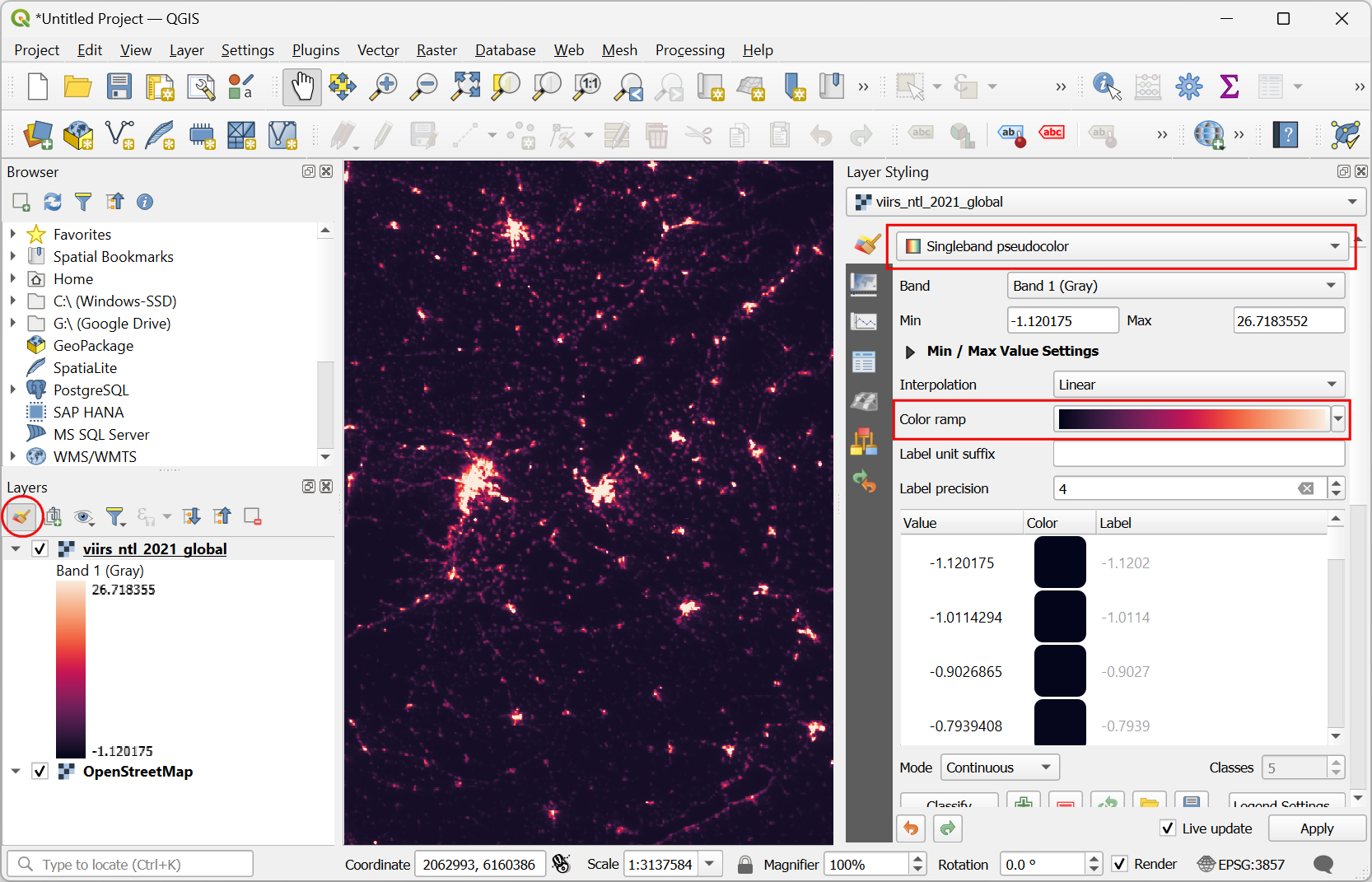
- In the Layer Styling panel, change the renderer to
Singleband pseudocolor. Select a color ramp of your choice. The layer rendering will be updated.
1.2 Load a FlatGeoBuf (FGB) Vector Layer
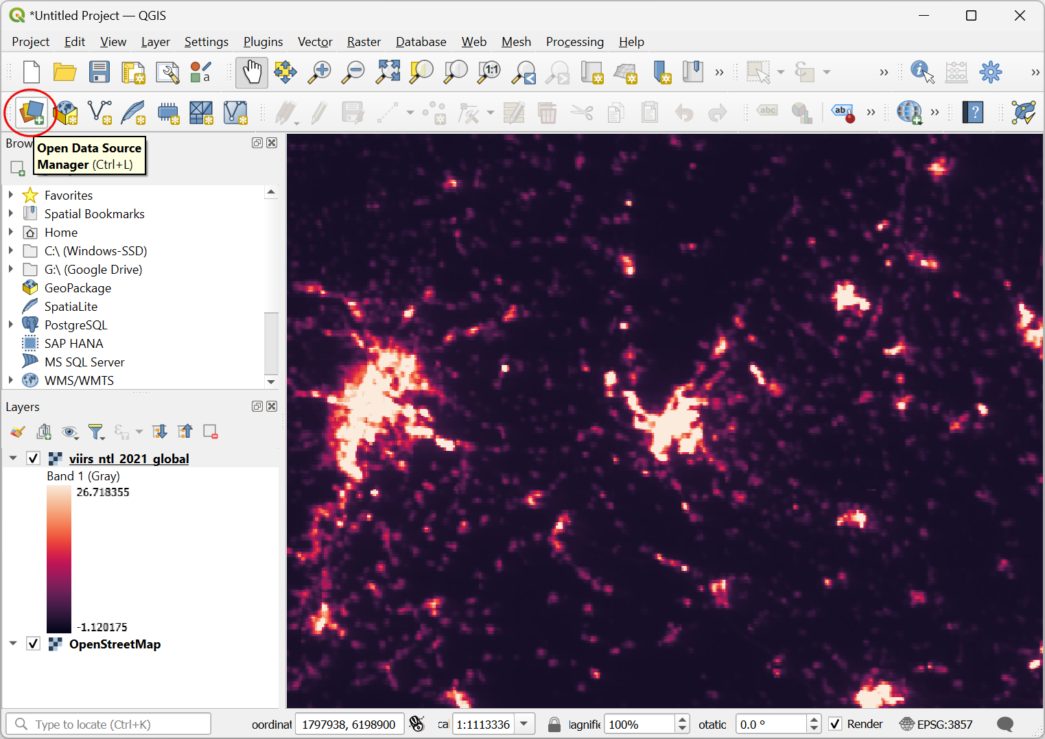
- Next, we will learn how to load a cloud-hosted vector layer to QGIS. We will stream a 800MB line layer hosted on GitHub file storage and stream the features in the current canvas extent. Click the Open Data Source Manager button.
- Select the Vector tab. Select
Protocol: HTTP(S), cloud etc.as the Source Type. Enter the following URL as the URI. Click Add.
https://github.com/spatialthoughts/cloud-native-geospatial/releases/download/hydrorivers/hydrorivers.fgb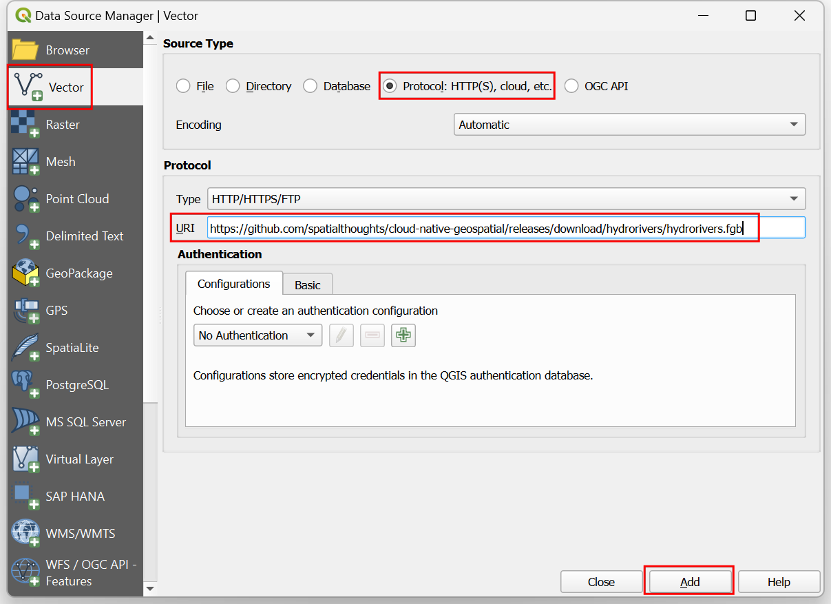
- A new layer
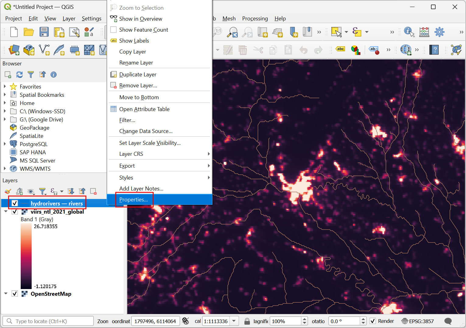
hydrorivers -- riverswill be added to the Layers panel. This is a large line layer containing over 2.5 million features. QGIS will request and load only the features within the current canvas extent. FlatGeoBuf format does not contain simplified versions of features that can be loaded at lower zoom levels. So if you zoom out to a large region, all the features within that region will be requested. To prevent fetching unnecessarily large amounts of data - we can enable scale dependent visibility. Right-click thehydrorivers -- riverslayer and select Properties.
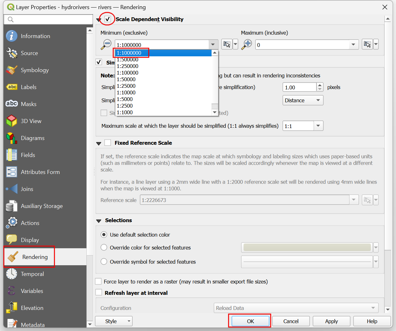
- Select the Rendering tab and enable the Scale Dependent
Visibility. From the drop-down selector for Minimum
(exclusive) scale, select
1:1000000. Click OK.
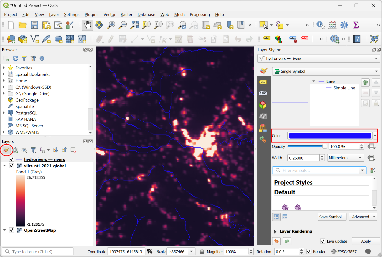
- Now only when your canvas is zoomed in beyond the selected scale, the features will be requested and rendered. Next, we will apply some style to the vector layer. Click the Open Layer Styling Panel button on the Layers panel. Change the Color to any color of your choice. You can also adjust the Width of the lines if required.
- Zoom/Pan around the map and go to any region in the world. Data from both the cloud-hosted files will be requested and rendered in the chosen style.
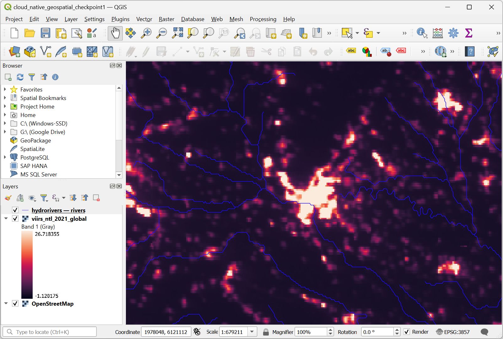
Your output should match the contents of the
cloud_native_geospatial_checkpoint1.qgz file in your data
package.
2. SpatioTemporal Asset Catalogs (STAC)
2.1 Explore STAC Catalogs
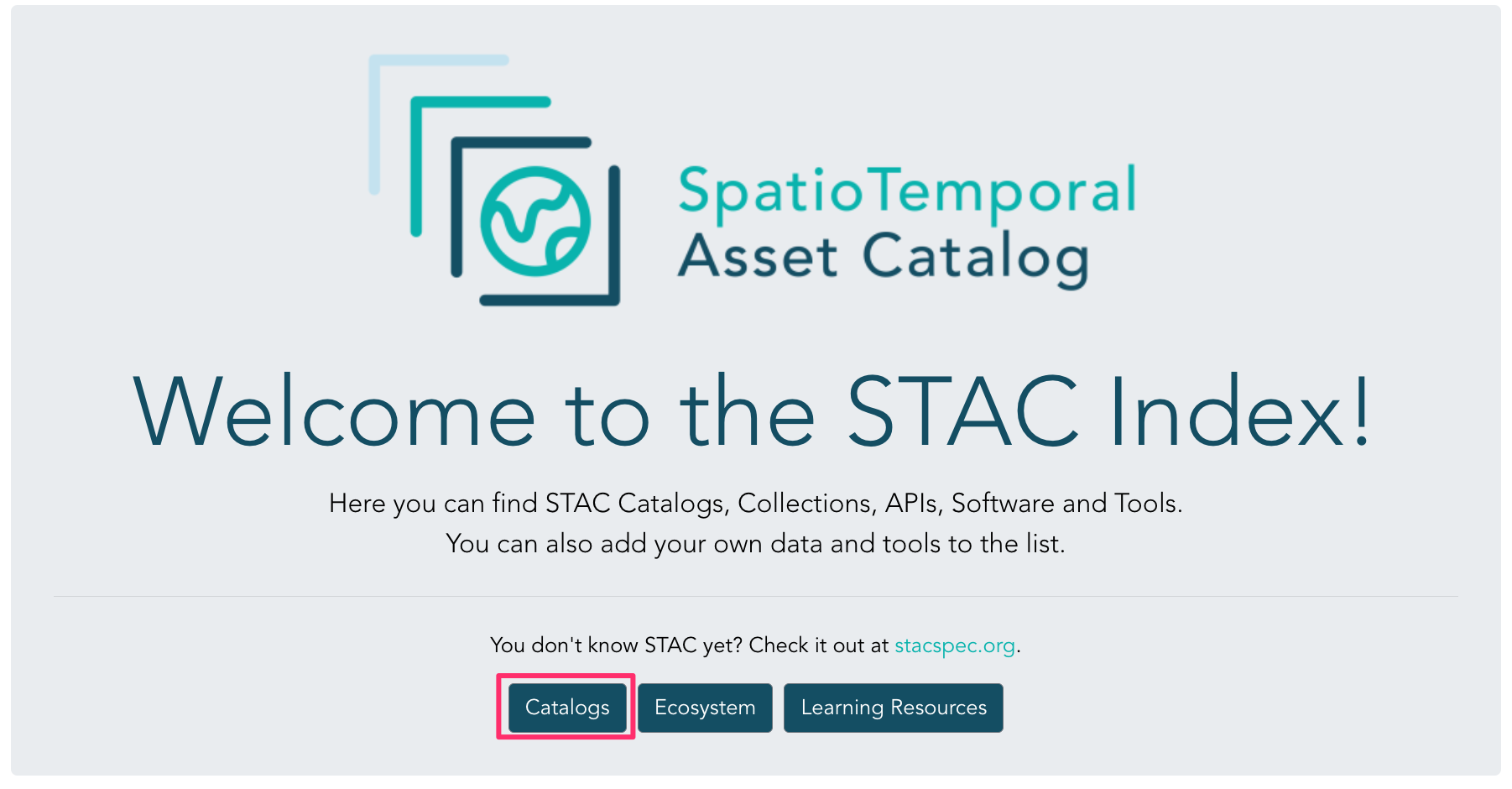
There are many publicly accessible STAC catalogs available - with more providers making their data available through STAC. To explore all the available catalogs, you can visit the STAC Index. Click on Catalogs and explore the listings.
2.2 Load a STAC Asset
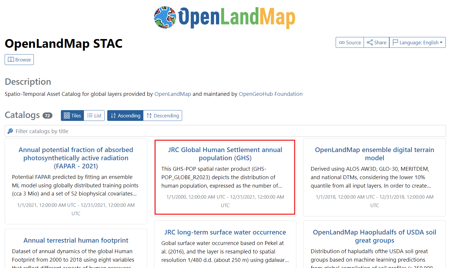
- Visit the OpenLandMap STAC catalog in a web browser. Locate the JRC Global Human Settlement annual population (GHS) collection and click to view more details.
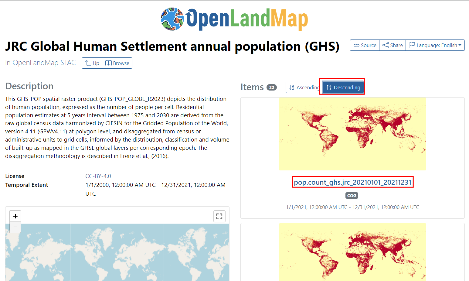
- This collection consists of GHSL Gridded Population rasters from year 2000-2021. Sort the collection in Descending order. The first item will be the latest population raster. Click on it to explore it further.
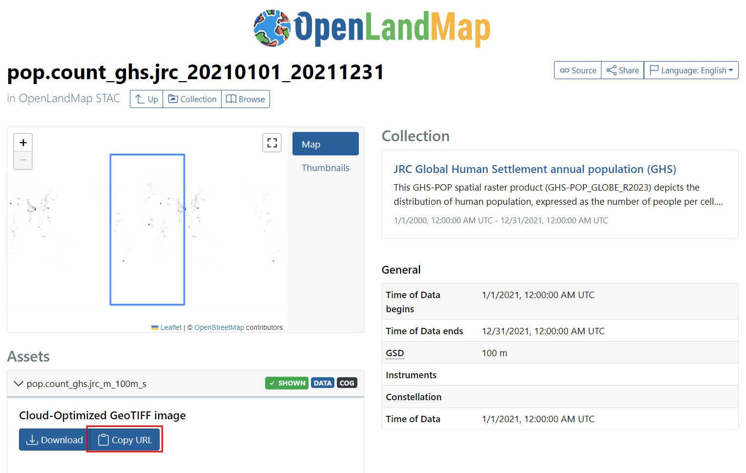
- This STAC Item consists of a Cloud-Optimized GeoTIFF image of population for the year 2021. Click Copy URL button to get the direct link to access the file.
- Open QGIS. From the Browser panel, scroll down and locate
XYZ Tiles → OpenStreetMap tile layer. Drag and drop it
to the main canvas. Once the
OpenStreetMaplayer is loaded, go to your region of interest. Click the Open Data Source Manager button.

- Select the Raster tab. Select
Protocol: HTTP(S), cloud etc.as the Source Type. Enter the URL copied in the previous step as the URI. Click Add.
https://s3.openlandmap.org/arco/pop.count_ghs.jrc_m_100m_s_20210101_20211231_go_epsg.4326_v20230620.tif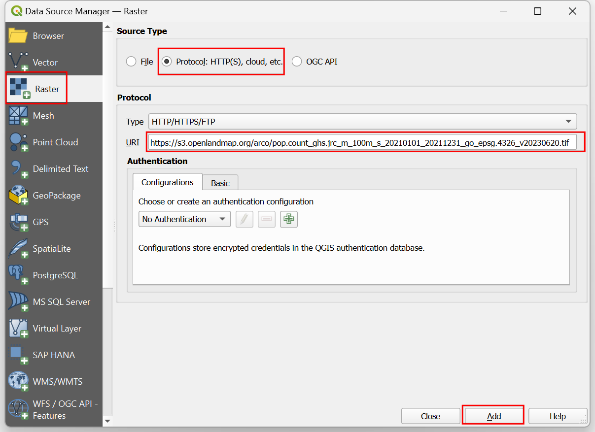
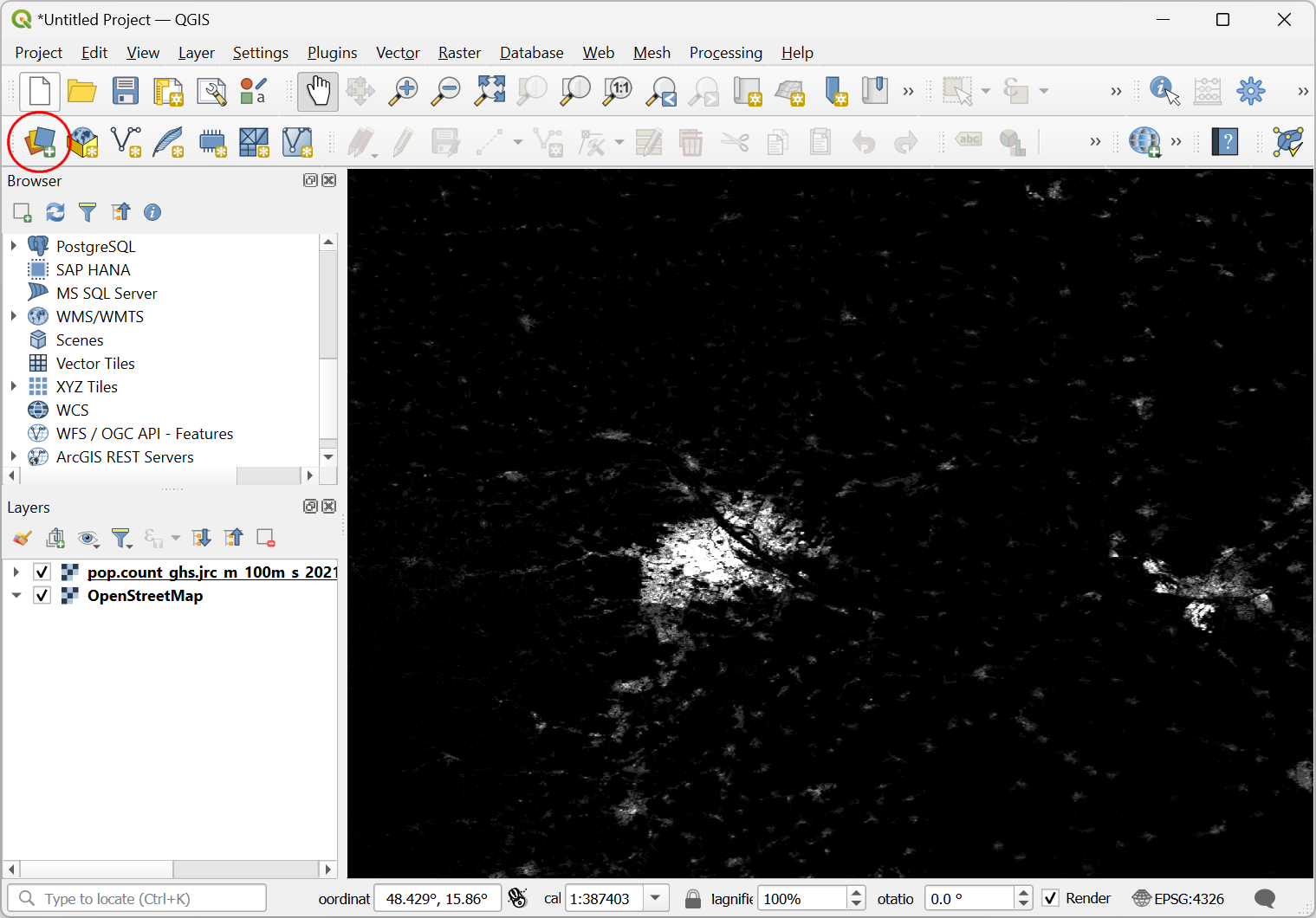
- A new layer
pop.count_ghs.jrc_m_100m_s_20210101_20211231_go_epsg.4326_v20230620will be added to the Layers panel. This image represents the population count in each 100m x 100m grid cell. The original data comes with decimal values, but to optimize the storage space and transfer of data, the image is saved with the data type UInt32 (Integers). To preserve the full fidelity of the data, the original pixel values are multiplied by 100. Hence if the the pixel value is2068- it represents a population count of20.68. Keep this in mind and we will appropriately scale our results with this factor.
2.3 Zonal Statistics with Cloud-hosted Data
- Let’s load some vector data. Click the Open Data Source
Manager button. Select the Vector tab. Select
Protocol: HTTP(S), cloud etc.as the Source Type. Enter the following URL as the URI. Click Add.
https://storage.googleapis.com/spatialthoughts-public-data/geoboundaries/admin2.fgb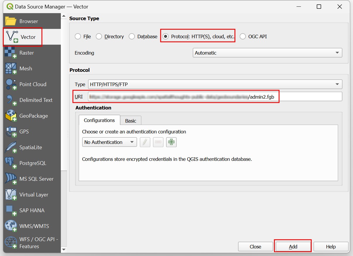
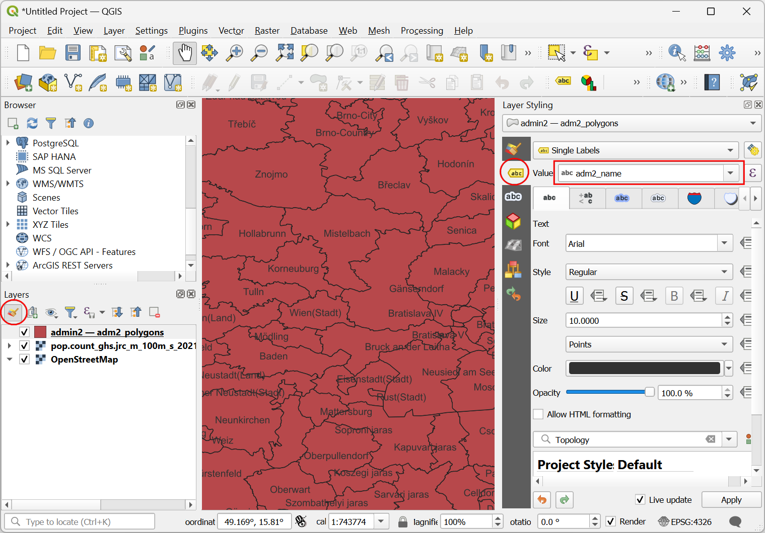
- A new layer
admin2 -- adm2_polygonswill be added to the Layers panel. This is a very large vector polygon layer and the polygons for Admin2 regions within the current canvas extents will be fetched and loaded. We will pick a region of interest. To make the selection easier, let’s add some labels to the polygons. Click the Open Layer Styling Panel button on the Layers panel.Select the Labels tab. SelectSingle Labelsfrom the drop-down menu and selectadm2_nameas the Value. The name of the administrative region will be rendered on the map.
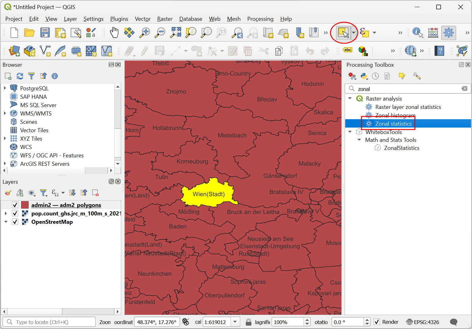
- Click on the Select Features by Area or Single Click button on the Selection Toolbar. Once activated, click on your chosen administrative region to select it. Go to Processing → Toolbox. From the Processing Toolbox, search and locate the Raster analysis → Zonal statistics algorithm. Double-click to open it.
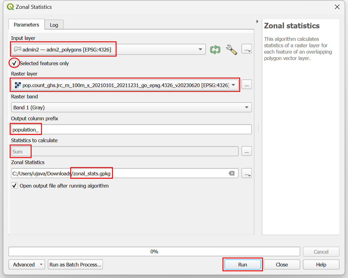
- In the Zonal Statistics dialog, select
admin2 -- adm2_polygonsas the Input layer. Make sure to check the Selected features only box. Select thepop.count_ghs.jrc_m_100m_s_20210101_20211231_go_epsg.4326_v20230620layer as the Raster layer. Enterpopulation_as the Output column prefix. For the Statistics to calculate, click the … button and select onlySum. Save the output as a filezonal_stats.gpkgand click Run.
- The algorithm will fetch the pixels required to perform the
calculation and once complete, a new layer
zonal_statswill be added to the Layers panel. This layer contains the result of the Zonal Statistics that was computed directed from the cloud-hosted dataset by fetching only required pixels and features - saving us time, bandwidth and storage.
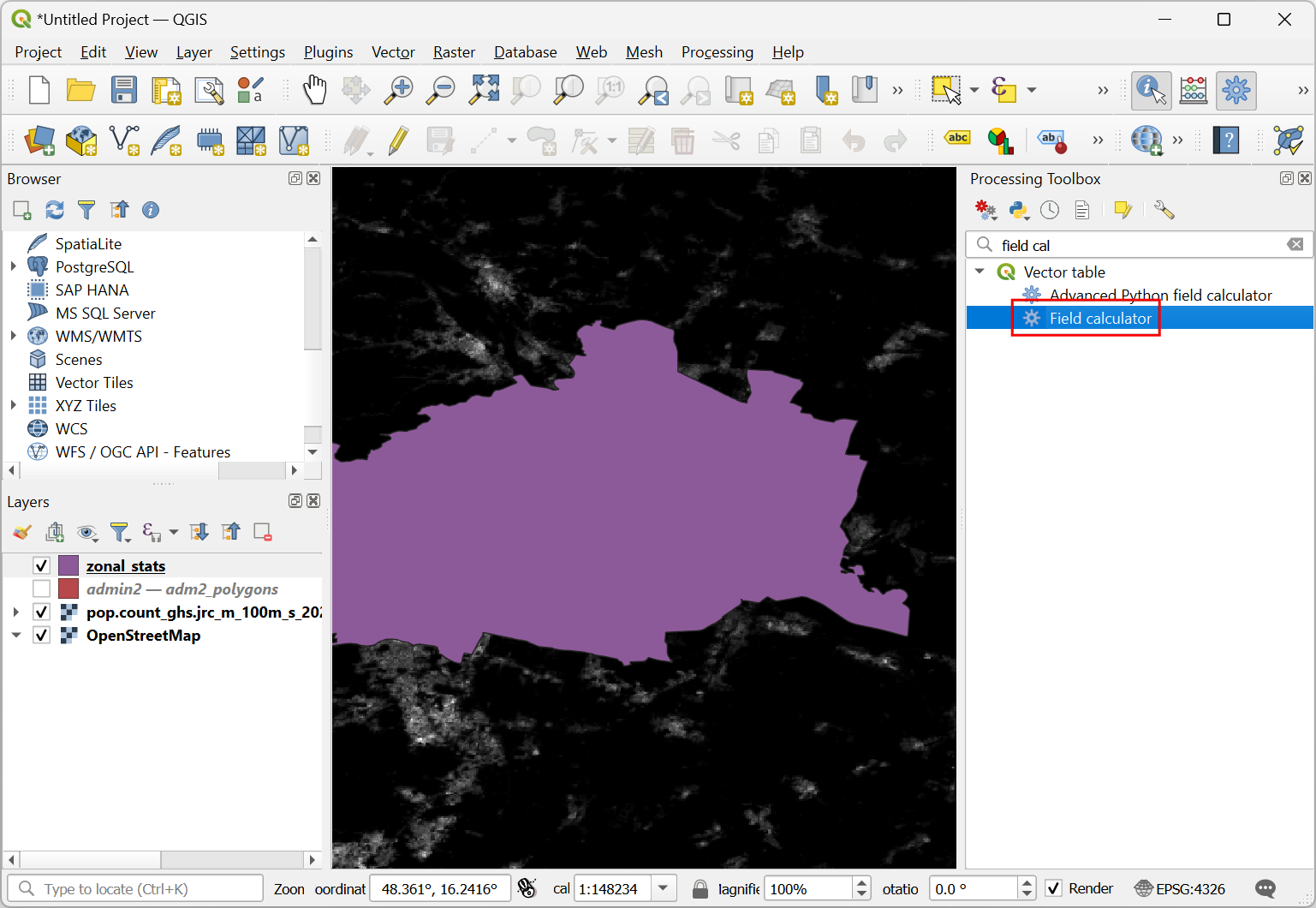
- The resulting value needs to be scaled by a factor of 100 to get the
actual population count. Search and locate the Vector table →
Field calculator algorithm and double-click to open it. Select
zonal_statsas the Input layer and enterpopulationas the Field name. Enter the following expression to scale the population value. Enter the output file name aszonal_stats_final.gpkgand click Run.
"population_sum" / 100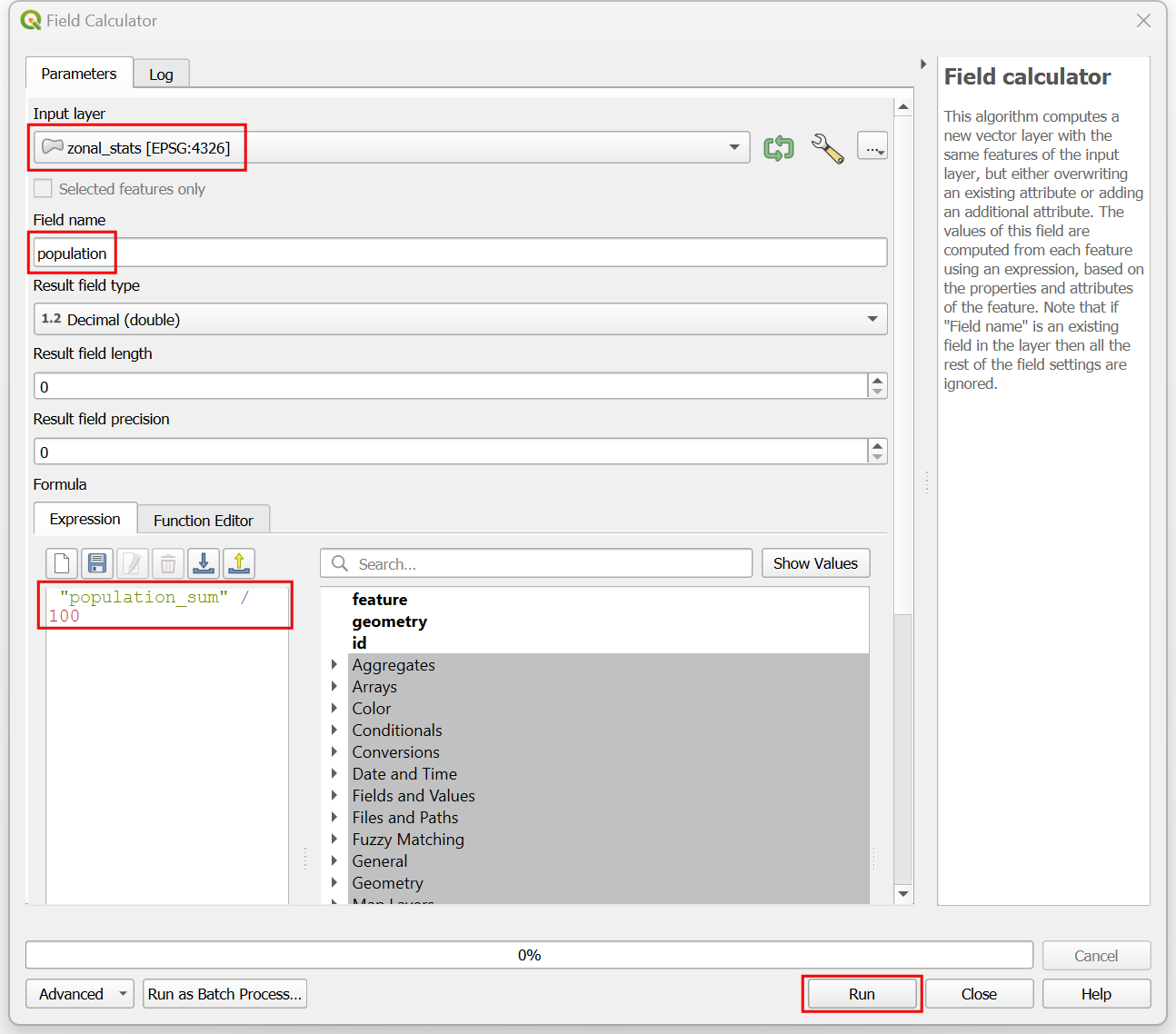
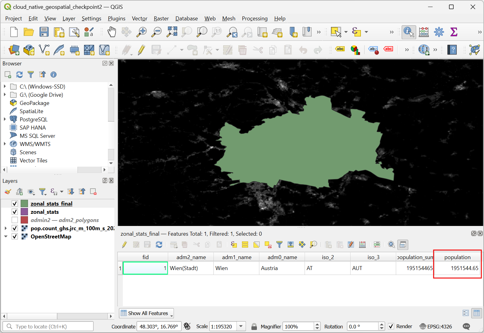
- Once the computation finishes and the new layer
zonal_stats_finalis loaded, right-click the layer and select Open Attribute Table. The field population contains the total population within the selected administrative region.
Your output should match the contents of the
cloud_native_geospatial_checkpoint2.qgz file in your data
package.
3. STAC API Browser Plugin
Note: The STAC API Browser plugin is no longer maintained. QGIS 3.44 includes native support for STAC that is being deveoped actively. [Learn more]. This section will be updated to use the native STAC provider once it matures.
3.1 Query a STAC API Catalog
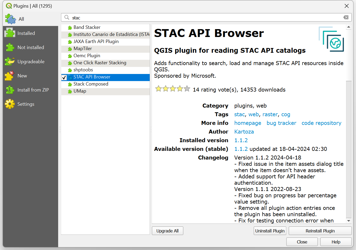
- Let’s install the STAC API Browser plugin. Go to
Plugins → Manage and Install Plugins. Select the
All tab and search for
STAC API Browser. Once you find the plugin, click Install.
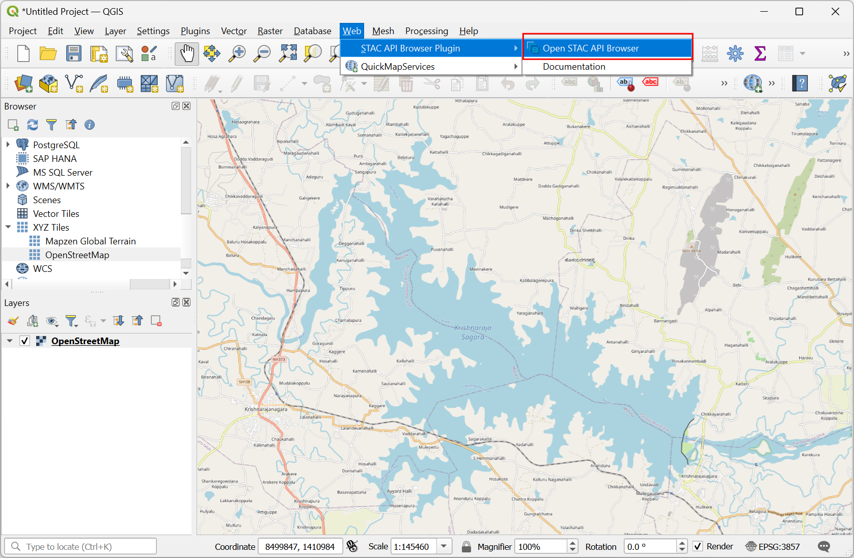
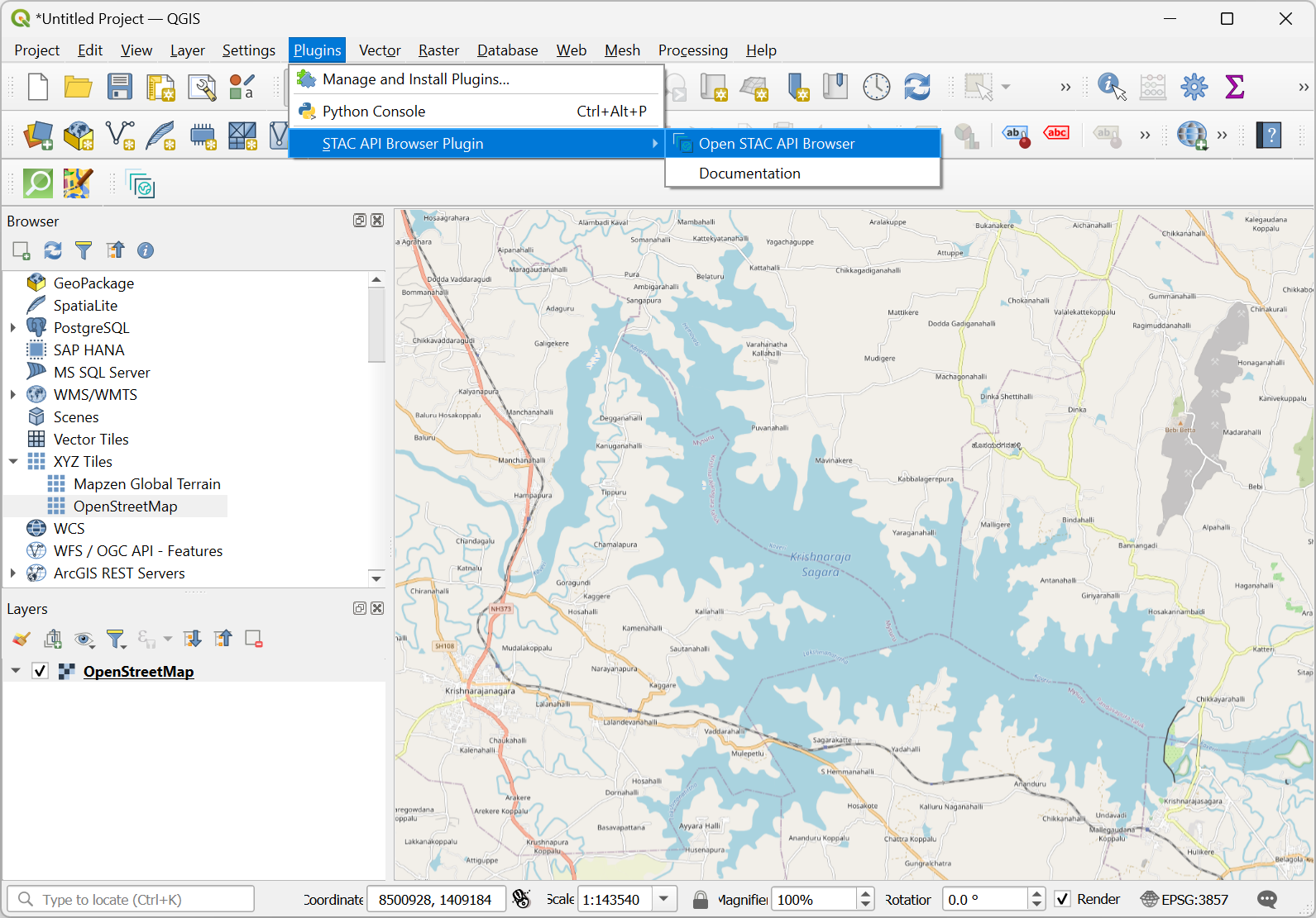
- Once installed, open the plugin from Web → STAC API Browser Plugin → Open STAC API Browser.
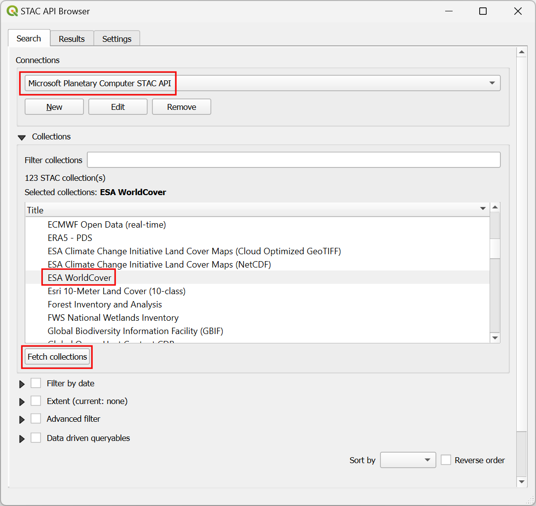
- In the STAC API Browser window, select
Microsoft Planetary Computer STAC APIas the Connections. Click Fetch collections to get all the collections available through the API. Scroll down and select theESA WorldCovercollection.
- In the same window, scroll down and check the Extent box. Click the Map Canvas Extent to load the current extent. Click Search.
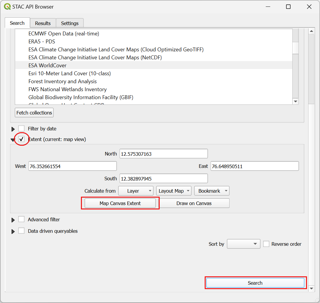
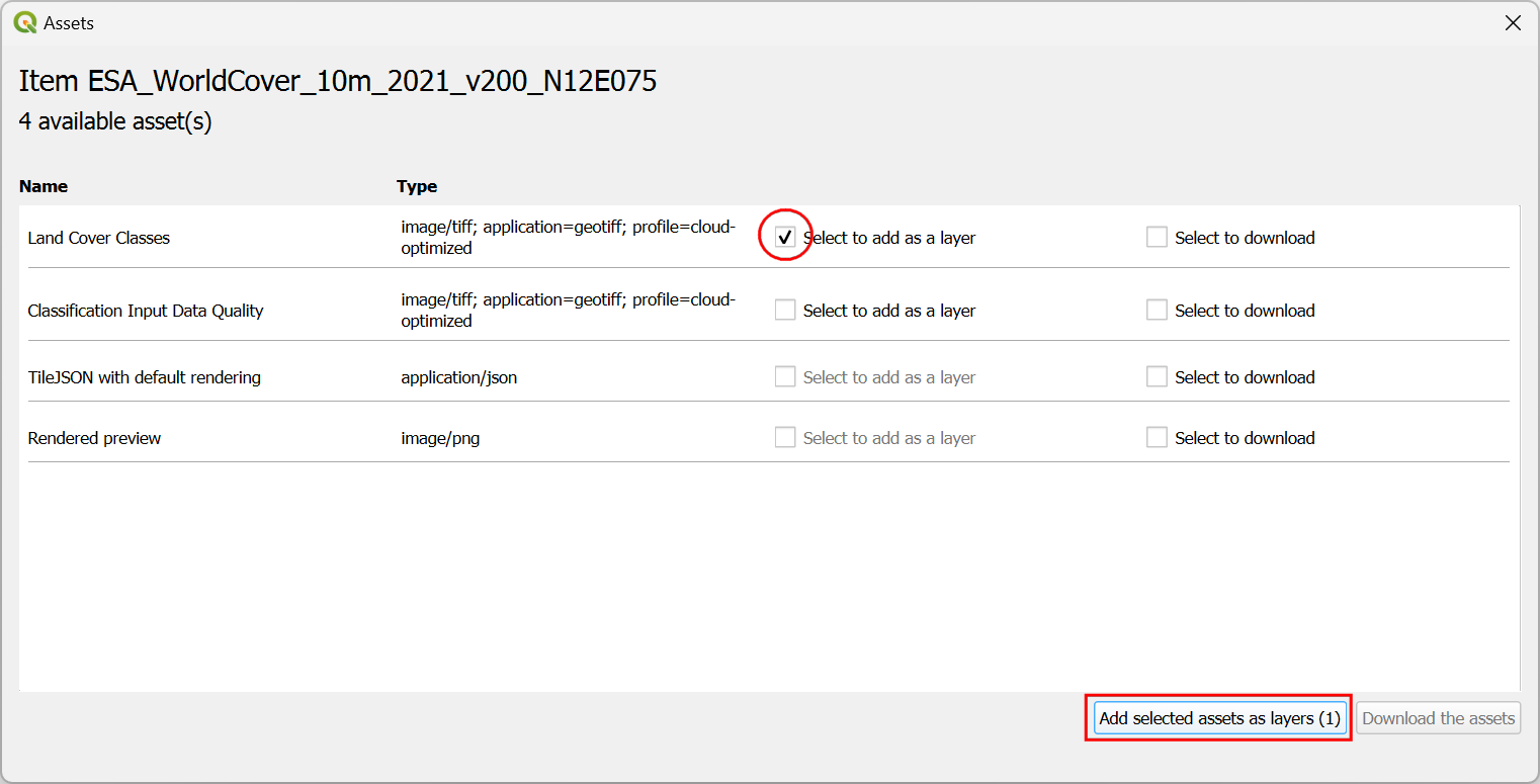
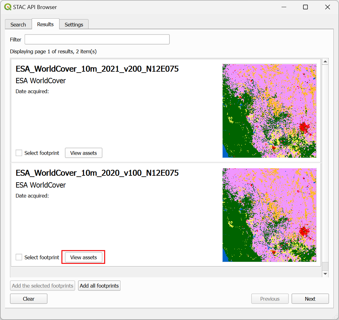
- This collection contains global landcover data for the years 2020 and 2021. The global dataset is split into several small tiles. You will see the matching tiles as items in the result. Click View assets for the item for the year 2021.

- We will load the
Land Cover Classesasset. Check the box Select to add as a layer and click Add select assets as layers.
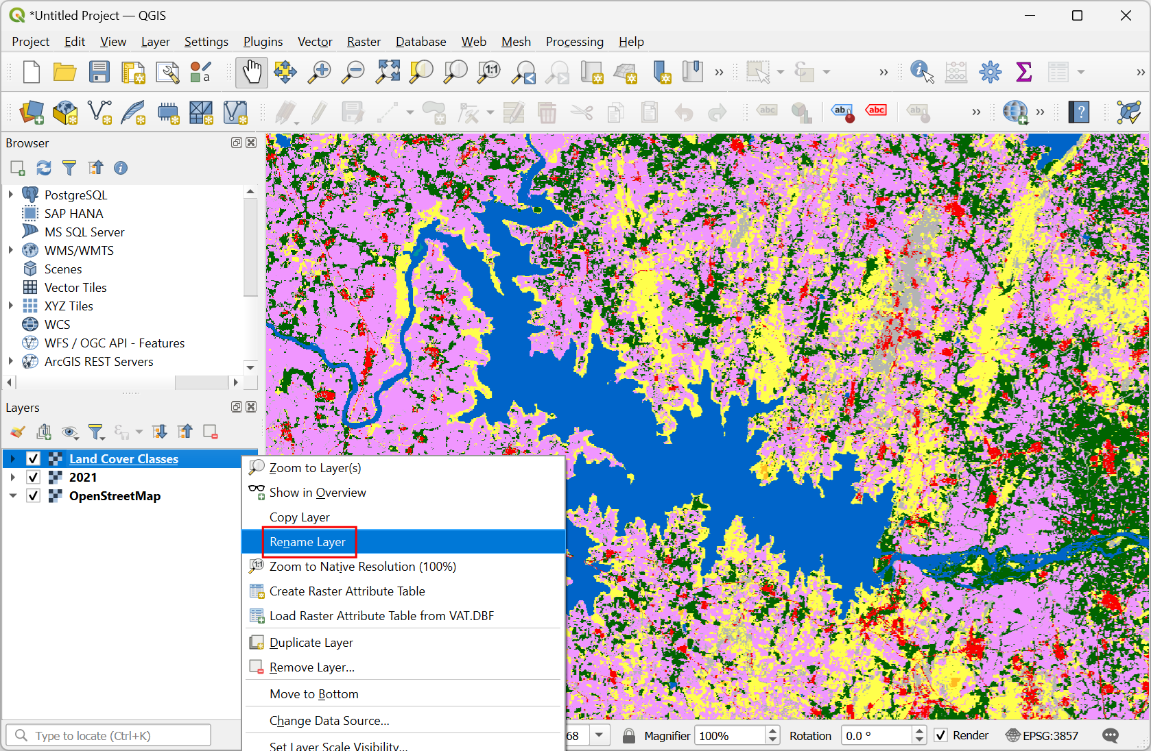
- A new layer
Land Cover Classeswill be added to the Layers panel and the landcover pixels for the region will be streamed in. Let’s rename the layer so we can easily identify it later. Right-click and select Rename Layer.
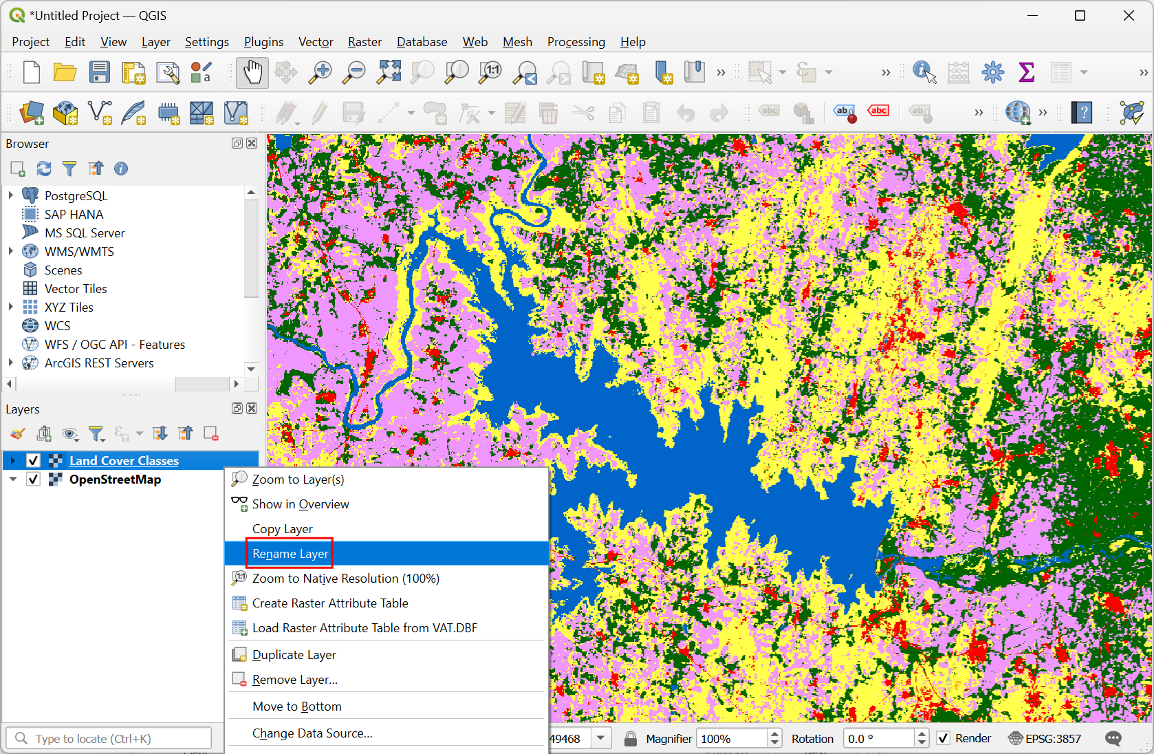
- Enter the layer name as
2021and press Enter.
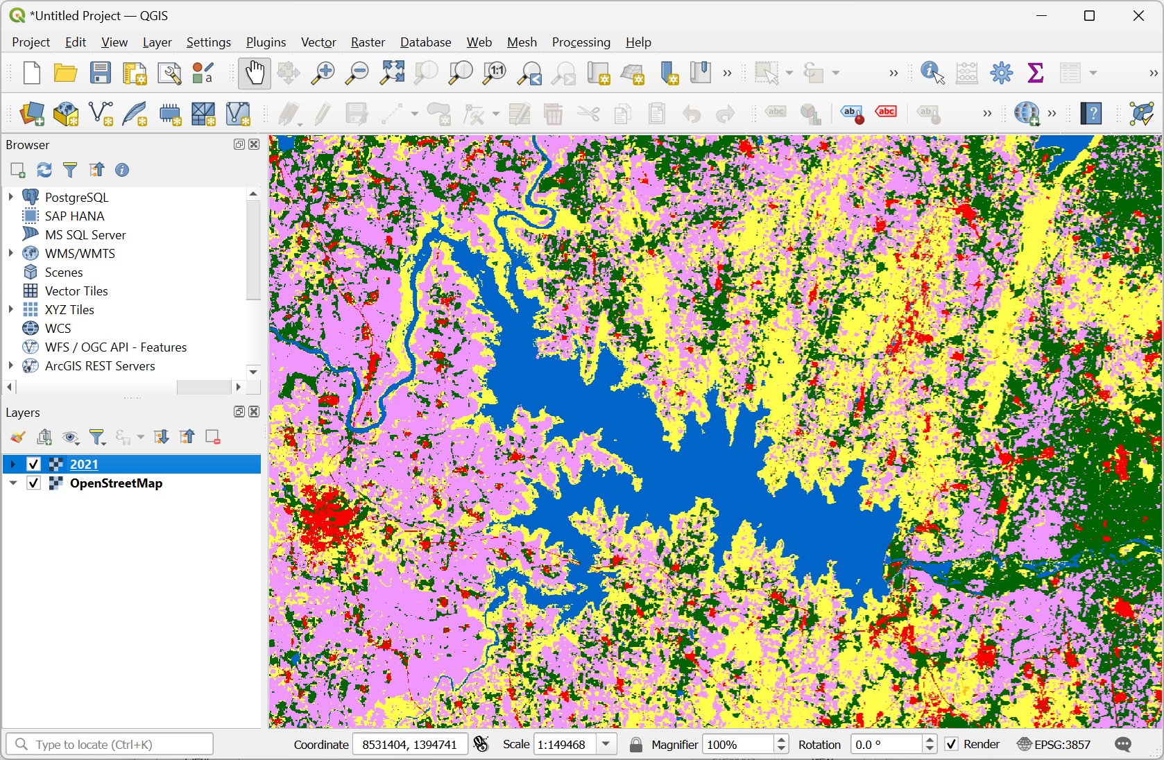
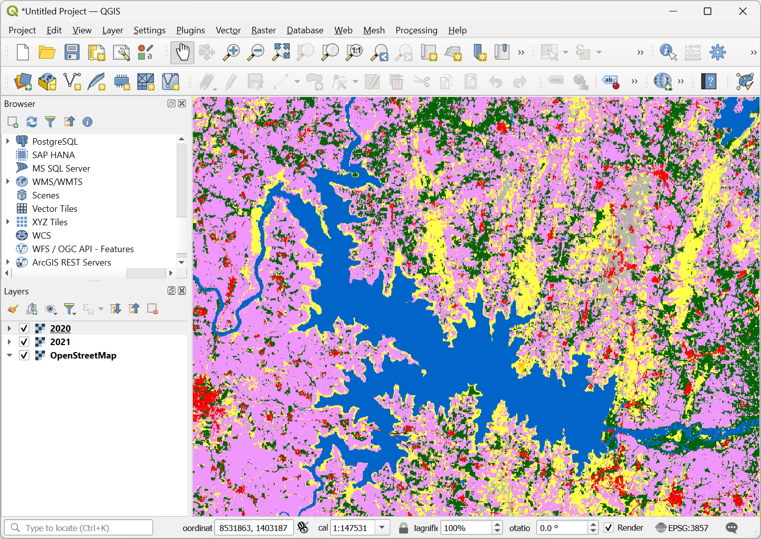
- Switch back to the STAC API Browser window and load the
Land Cover Classesasset for the year 2020.
- Once the layer is loaded, rename it to
2020.
- We queries and successfully loaded 2 remote layers for the landcover classification for the year 2020 and 2021.
3.2 Analyze Landcover Change
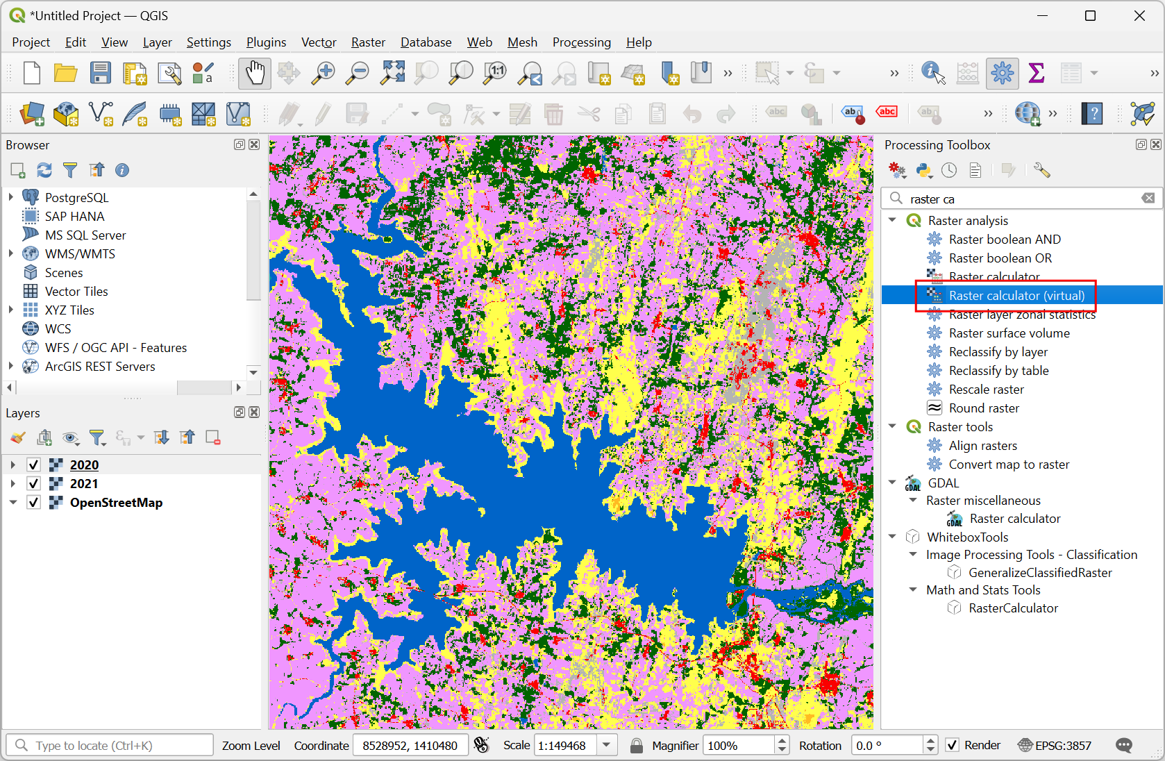
We will now analyze the change in water class between the year 2020 and 2021 to locate all areas where surface water was lost.
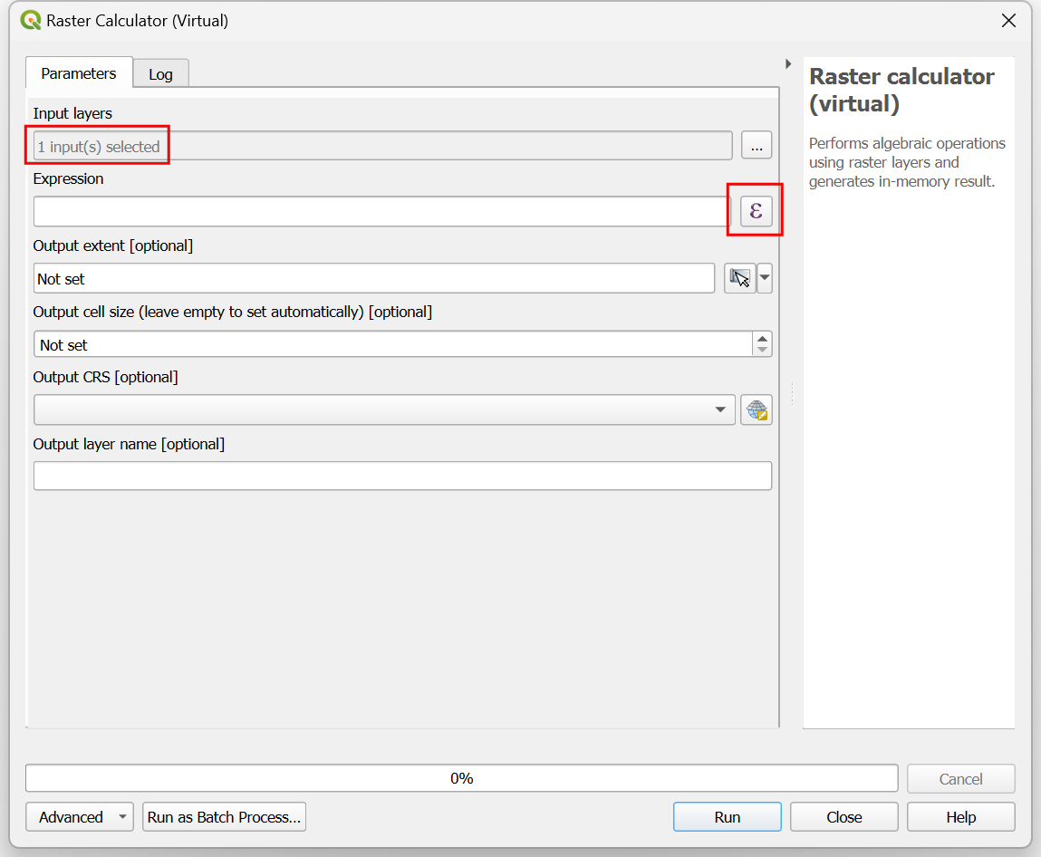
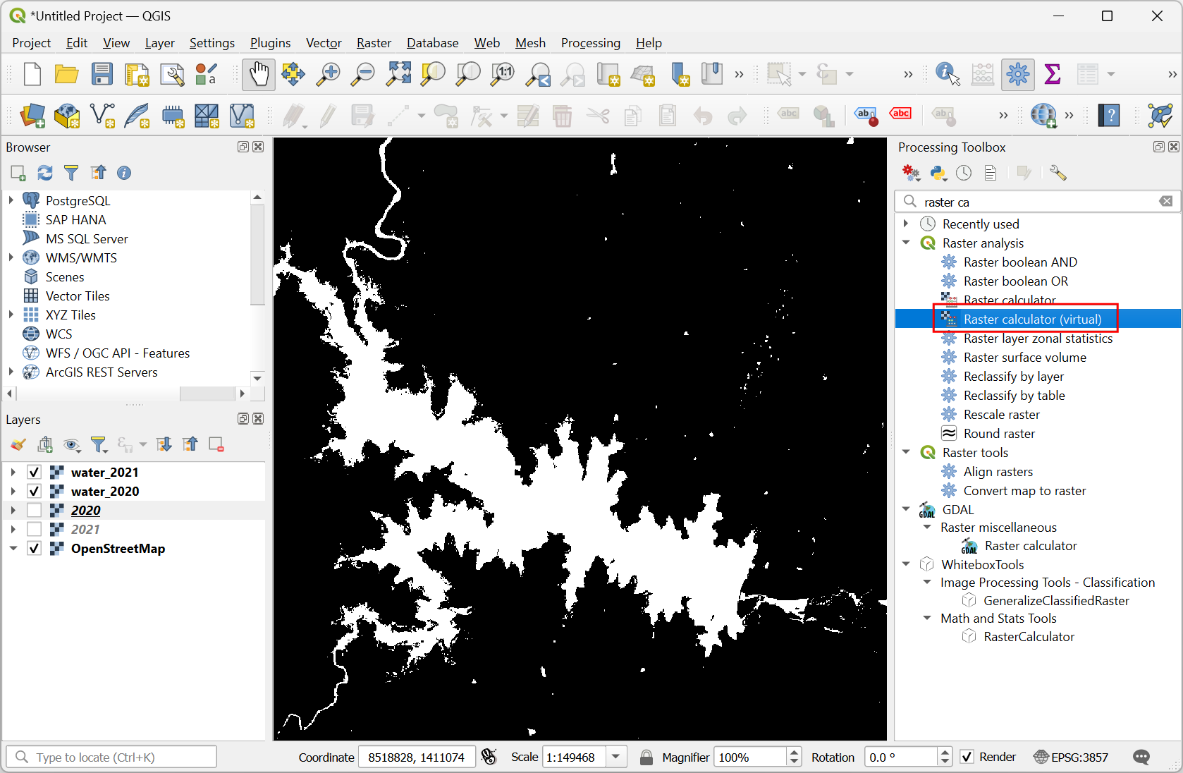
- To perform raster algebra on cloud layers, we need to use a special version of the raster calculator. Open the Processing Toolbox from Processing → Toolbox. Search and locate the Raster analysis → Raster calculator (virtual). Double-click to open it.
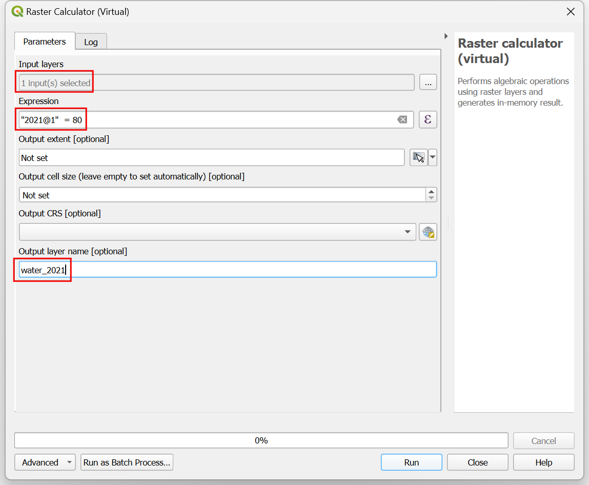
- In the Raster calculator (virtual) dialog, click the
… button next to Input layers and select the
2020layer. Next click the Expression button.
- ESA WorldCover classification assigns the pixel value 80 to Permanent Water Bodies View Documentation. Enter the following expression to select all pixels classified as water. Click OK.
"2020@1" = 80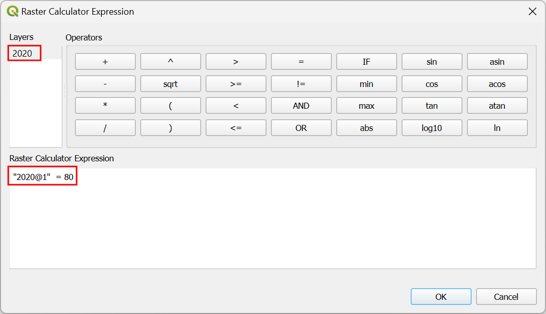
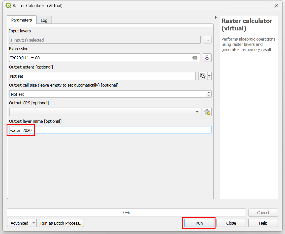
- Back in the Raster calculator (virtual) dialog, enter
water_2020as the Output layer name and click Run.
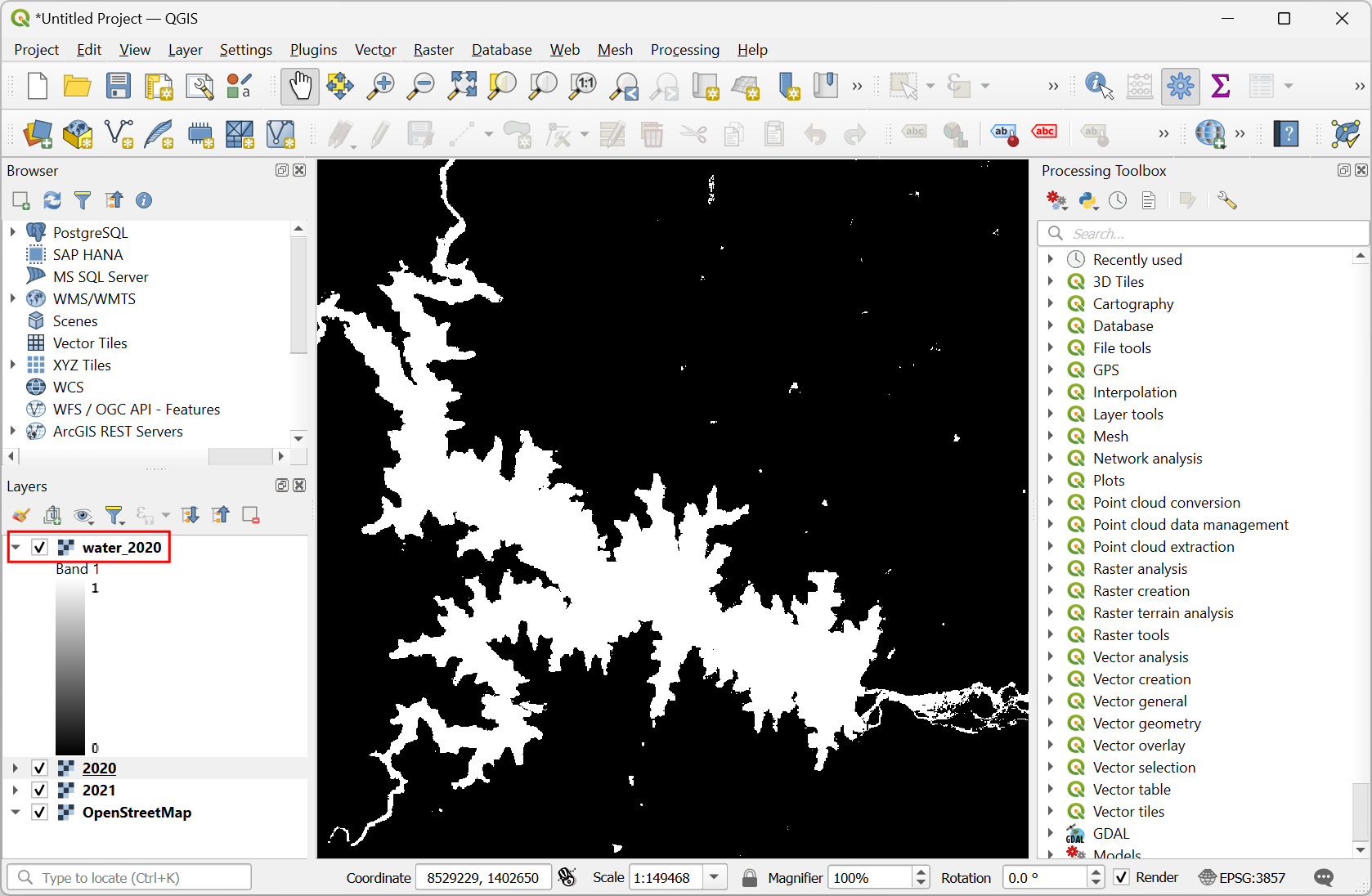
- A new layer
water_2020will be added to the Layers panel. This is a boolean layer with pixel values 1 for water and 0 for all other classes.
- Repeat the process for the 2021 layer. This time enter
water_2021as the Output layer name.
- We have now isolated the water pixels for both the years. Let’s analyze the change between the years. Search and locate the Raster analysis → Raster calculator (virtual). Double-click to open it.
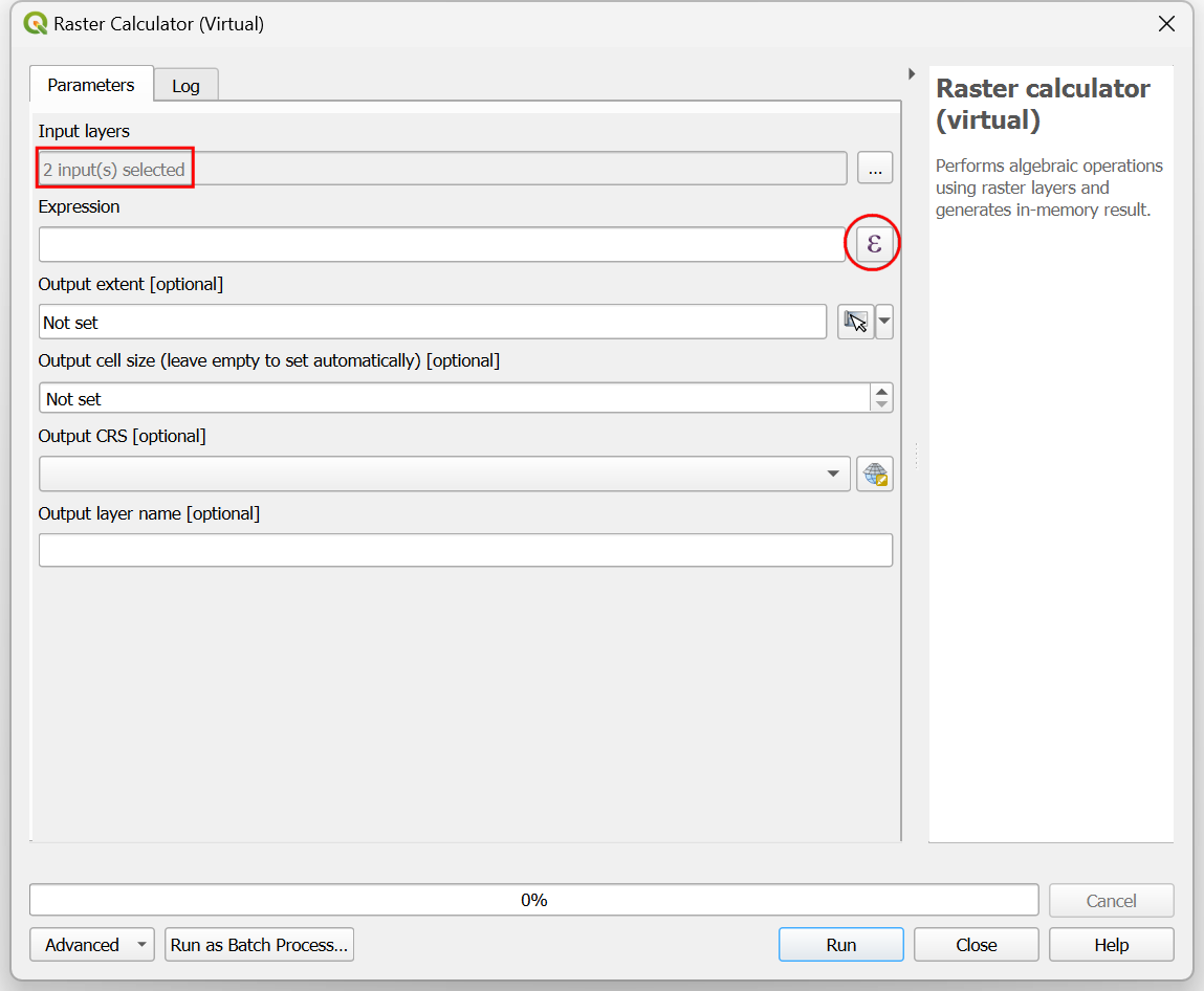
- In the Raster calculator (virtual) dialog, click the
… button next to Input layers and select both the
water_2020andwater_2021layers. Next click the Expression button.
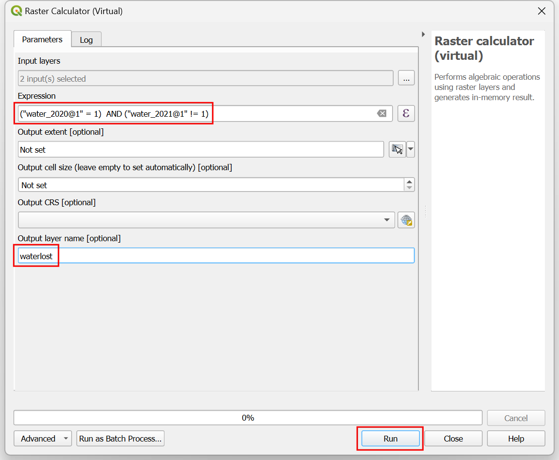
- We want to identify the loss in surface water. This can be done by selecting all pixels which were water in 2020 but not water in 2021. Enter the following expression to match these pixels.
("water_2020@1" = 1) AND ("water_2021@1" != 1)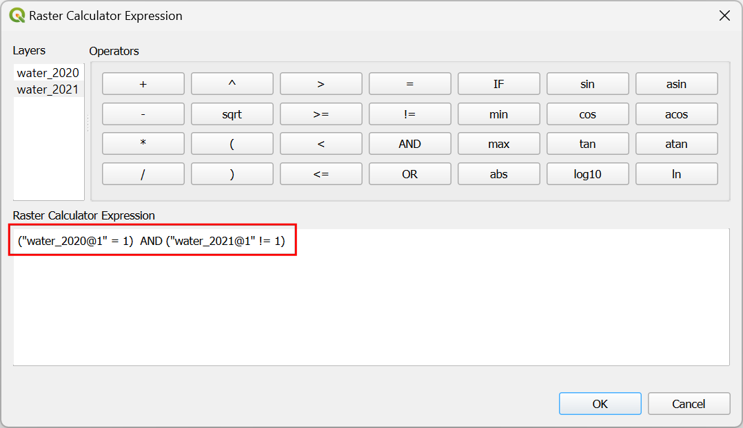
- Back in the Raster calculator (virtual) dialog, enter
waterlostas the Output layer name and click Run.
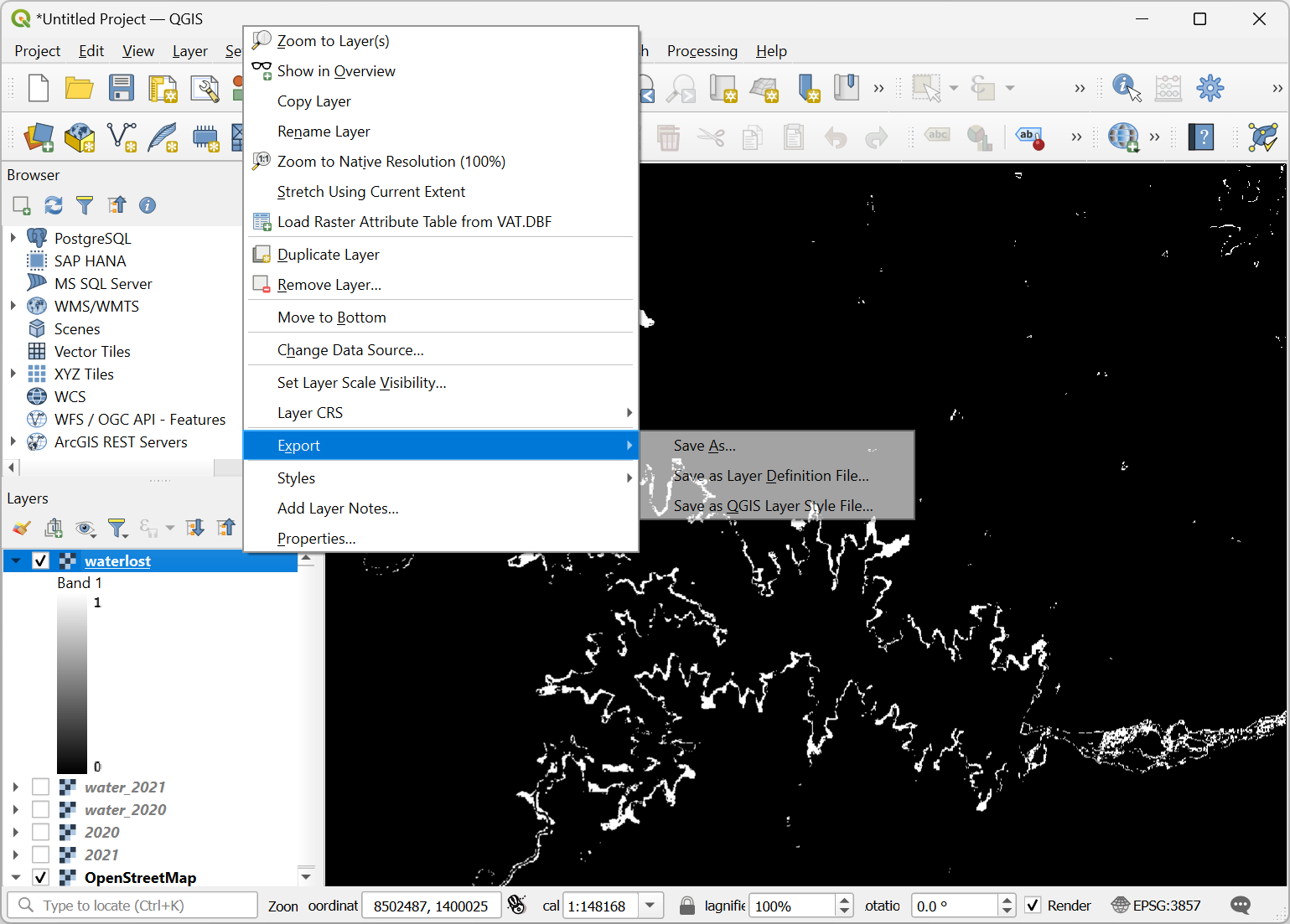
- A new layer
waterlostwill be added to the Layers panel. Everything we have done so far is a dynamic computation on the remote data layers. Let’s perform the actual computation and save the results as a local raster. Right-click thewaterlostlayer and go to Export → Save As….
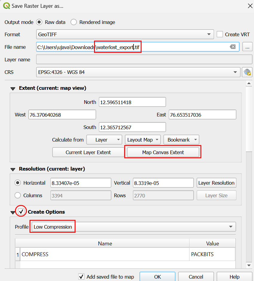
- In the Save Raster Layer as… dialog, click the …
button and browse to a folder on your computer. Enter
waterlost_export.tifas the output file name. Expand the Extent section and click the Map Canvas Extent button to load the current extent. It is always a good idea to apply a lossless compression to raster files. Check the Create Options box and selectLow Compressionas the Profile.
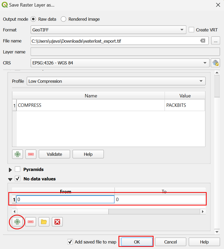
- Scroll down and check the No data values box. Click the
+ button and enter the values
0as From and To. This will only keep the pixels with value 1 as data values in the output. Click OK.
- QGIS will now request the pixels within the given extent and perform
the calculations as requested. It may take a few minutes depending on
the size of the region and available internet bandwidth. Once complete,
a new layer
waterlost_exportwill be added to the Layers panel.
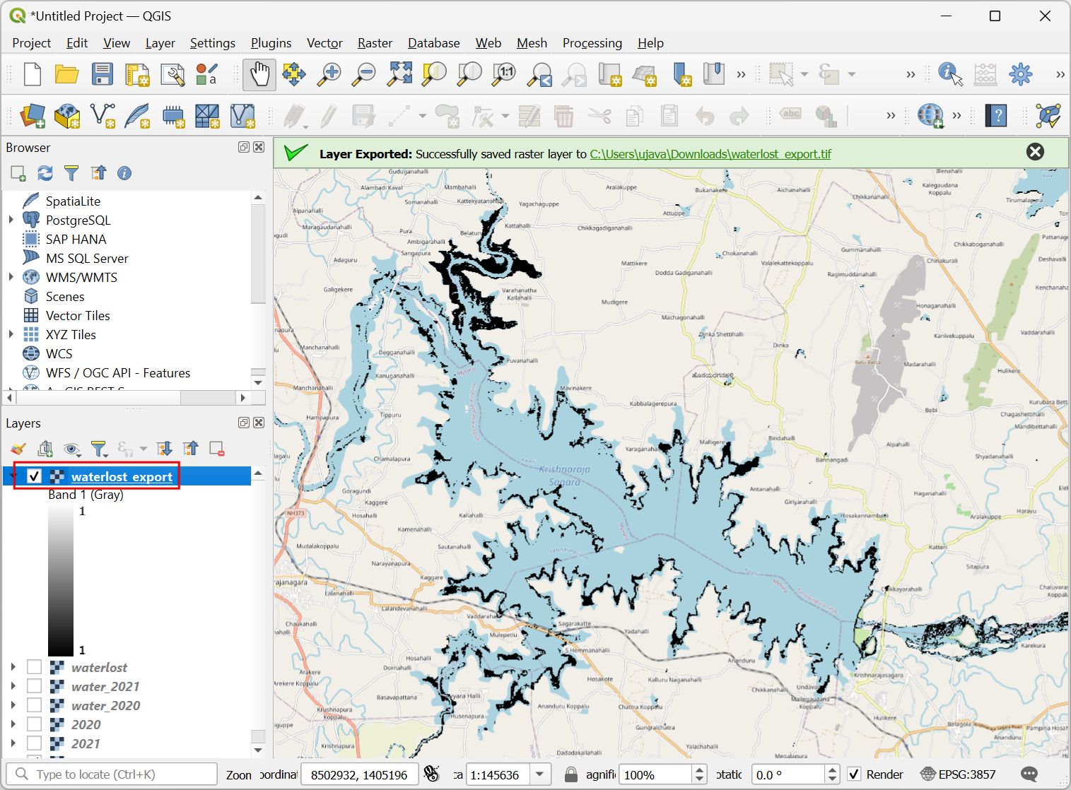
- The
waterlost_exportis a local raster with pixels showing regions that experienced loss in surface water. Let’s convert this layer to polygons. From the Processing Toolbox, search and locate the GDAL → Raster Conversion → Polygonize (raster to vector) algorithm.
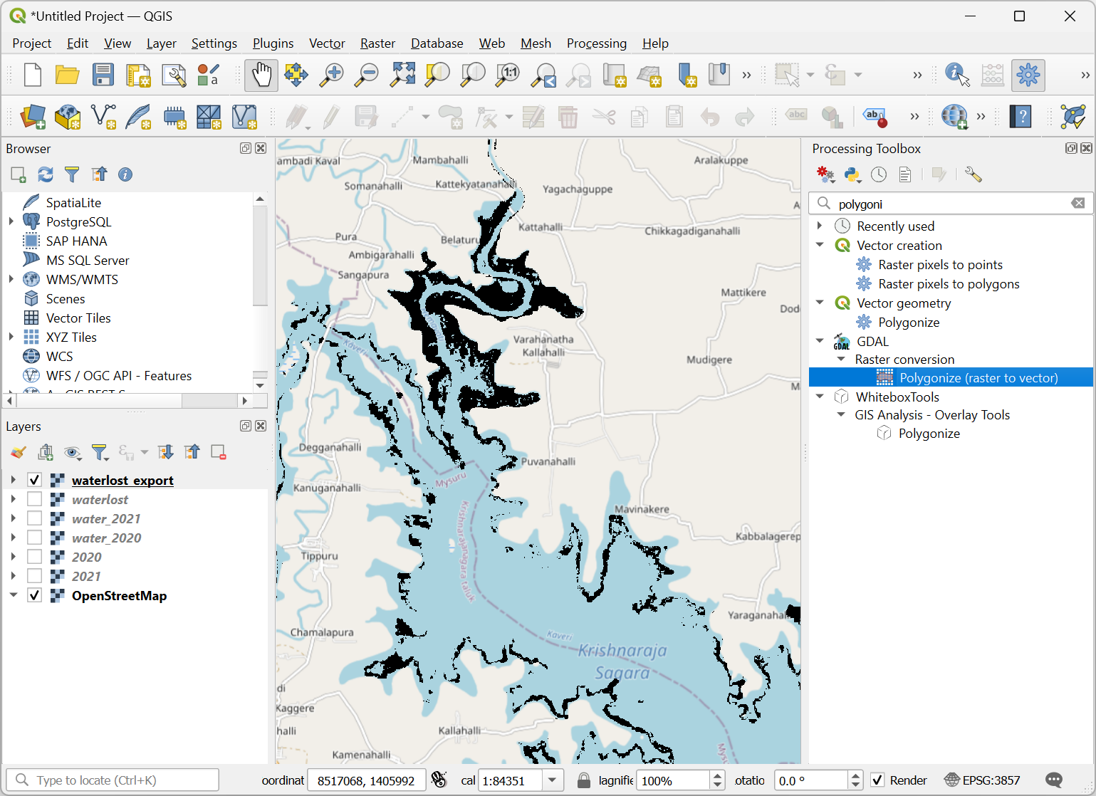
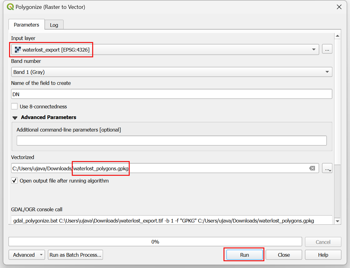
- In the Polygonize (raster to vector) dialog, select
waterlost_exportas the Input layer. Keep all other parameters to their default values. Click … next to Vectorized and browse to a folder on your computer. Enter the filename aswaterlost_polygons.gpkg. Click Run.
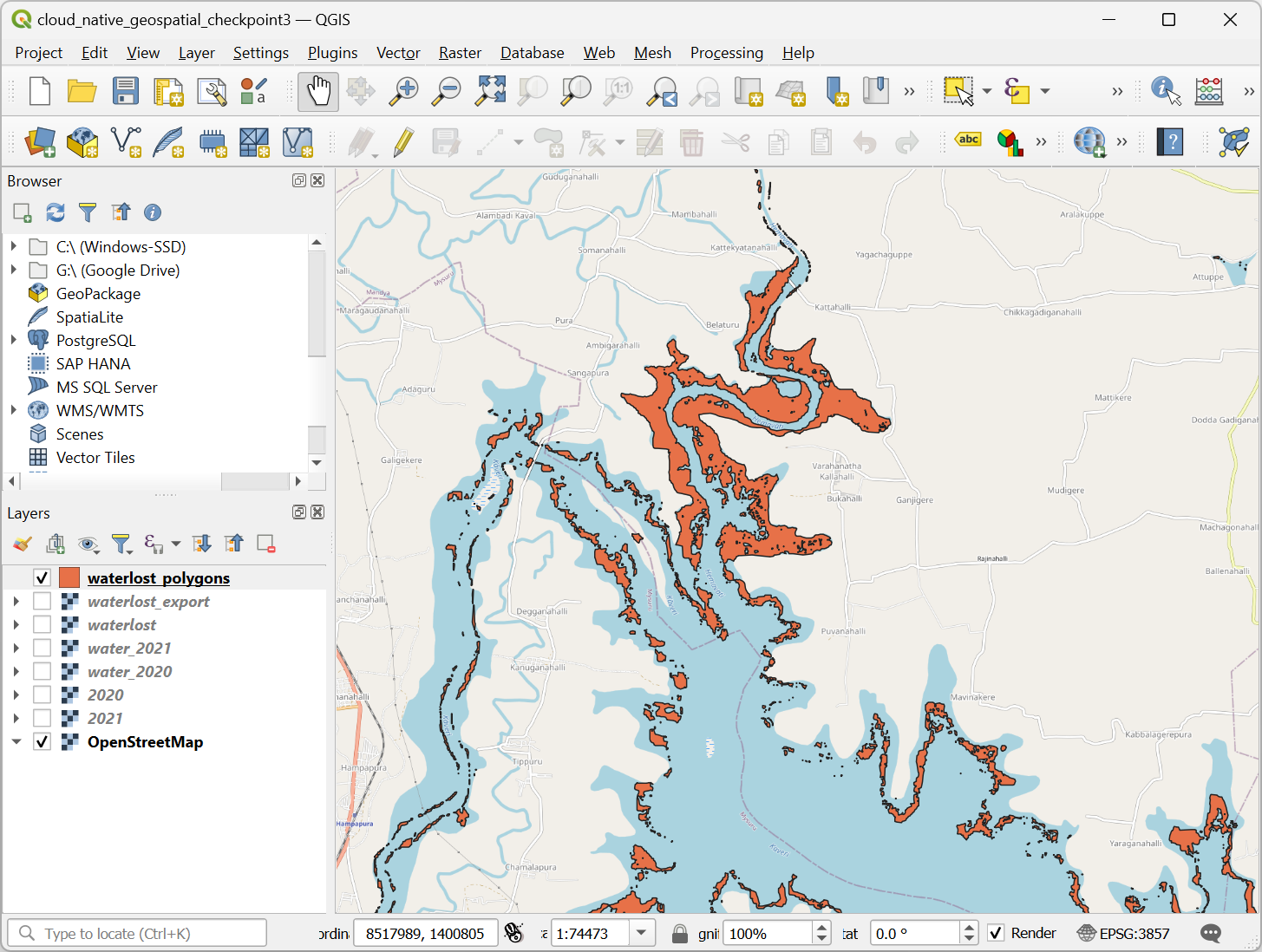
- Once the conversion is complete, a new layer
waterlost_polygonswill be added to QGIS. Using a cloud-native workflow, we were able to do a landcover change analysis without downloading any data or incurring any cloud computation cost.
Your output should match the contents of the
cloud_native_geospatial_checkpoint3.qgz file in your data
package.
4. Working with Cloud-Hosted Satellite Imagery
In this section, we will learn how to query a STAC catalog of Sentinel-2 L2A data, load and create a RGB composite and compute a spectral index using a cloud-native approach.
4.1 Loading Bands and Creating a RGB Composite
- Start by loading a basemap. From the Browser panel, scroll down and locate XYZ Tiles → OpenStreetMap tile layer. Drag and drop it to the main canvas. Zoom to your region of interest. We will use the STAC API Browser plugin to query for satellite images over this area. Open the plugin from Plugins → STAC API Browser Plugin → Open STAC API Browser.
- Select
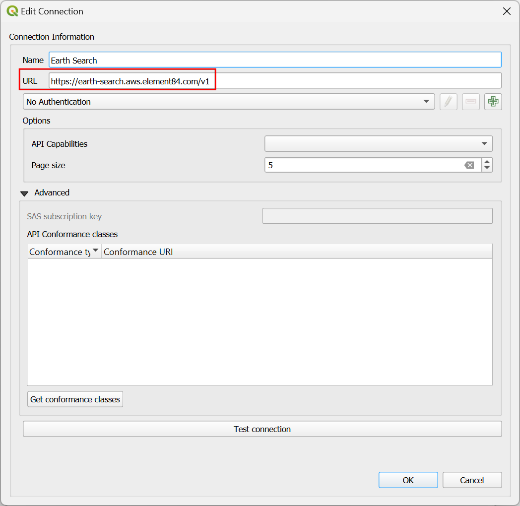
Earth Searchfrom the Connections dropdown. Click Edit to view the connection details.

- Make sure the URL is
https://earth-search.aws.element84.com/v1and click OK.
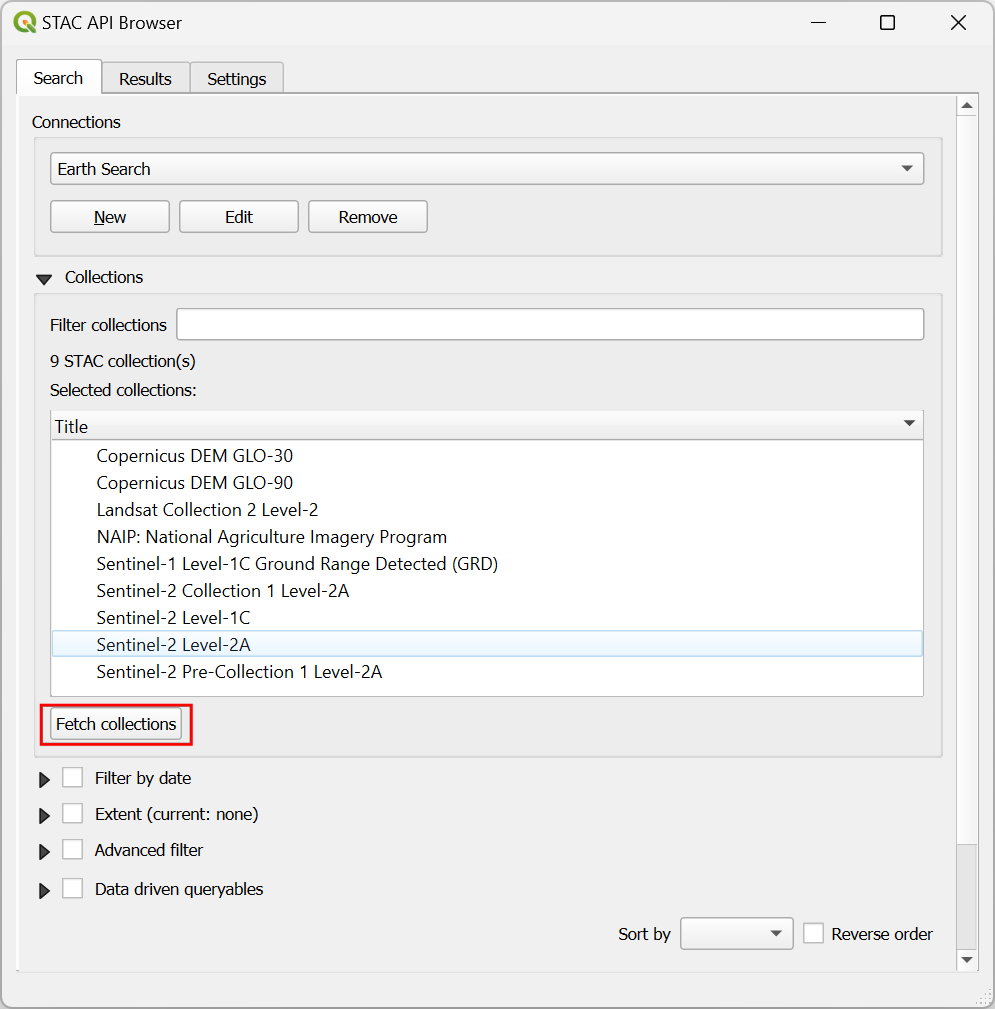
- In the STAC API Browser window, click the Fetch
collections button. Once the list updates, select the
Sentinel-2 Level-2Acollection. If you do not see this dataset listed, please go to the previous step and verify the URL is correct.
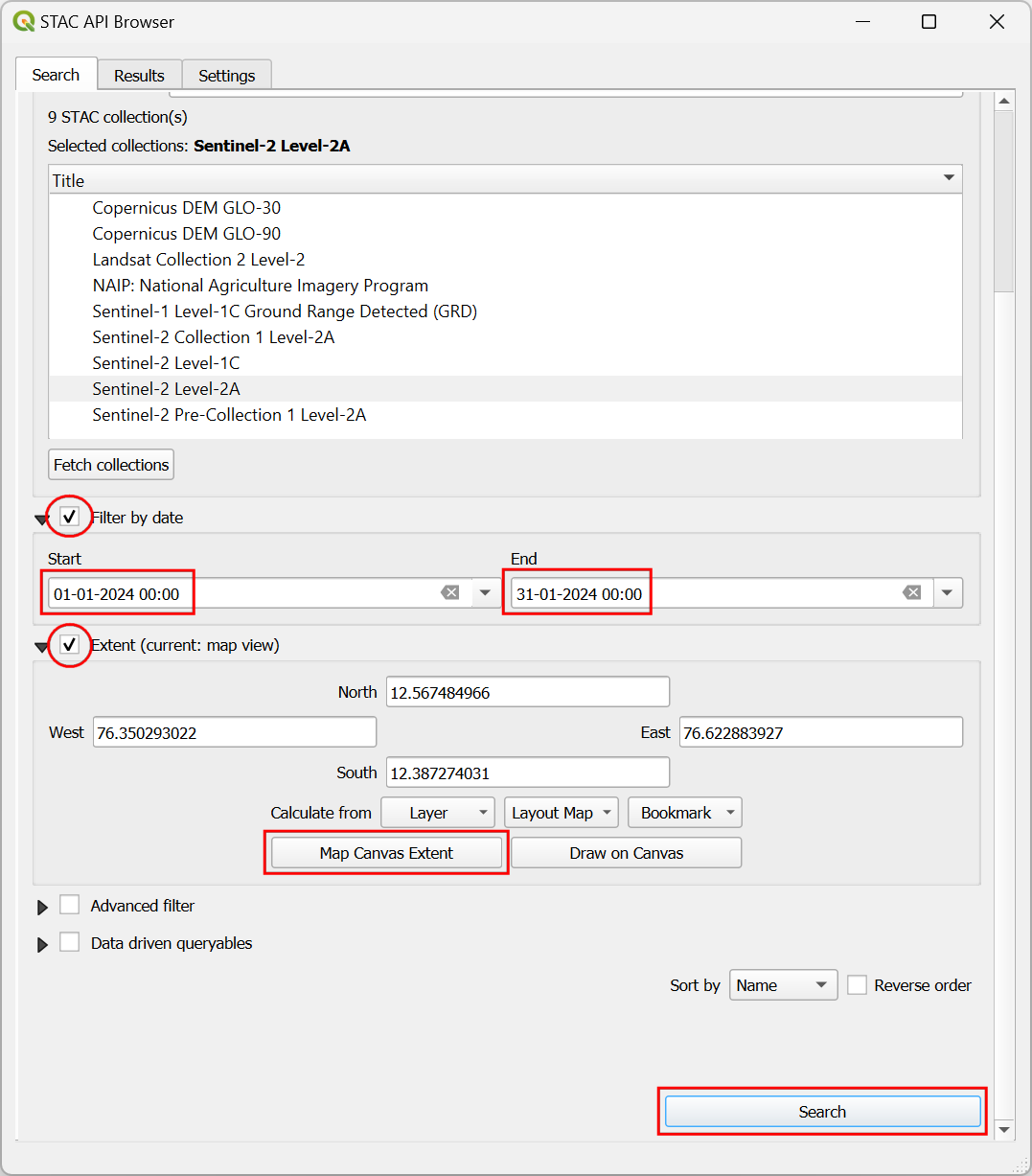
- Check the Filter by date option and enter a start and end date. Sentinel-2 Level-2A dataset is available from 2017 onward and a new image is collected every 5 days. Check the Extent option and click Map Canvas Extent button to fill the coordinates of the region visible on the map. Click Search.
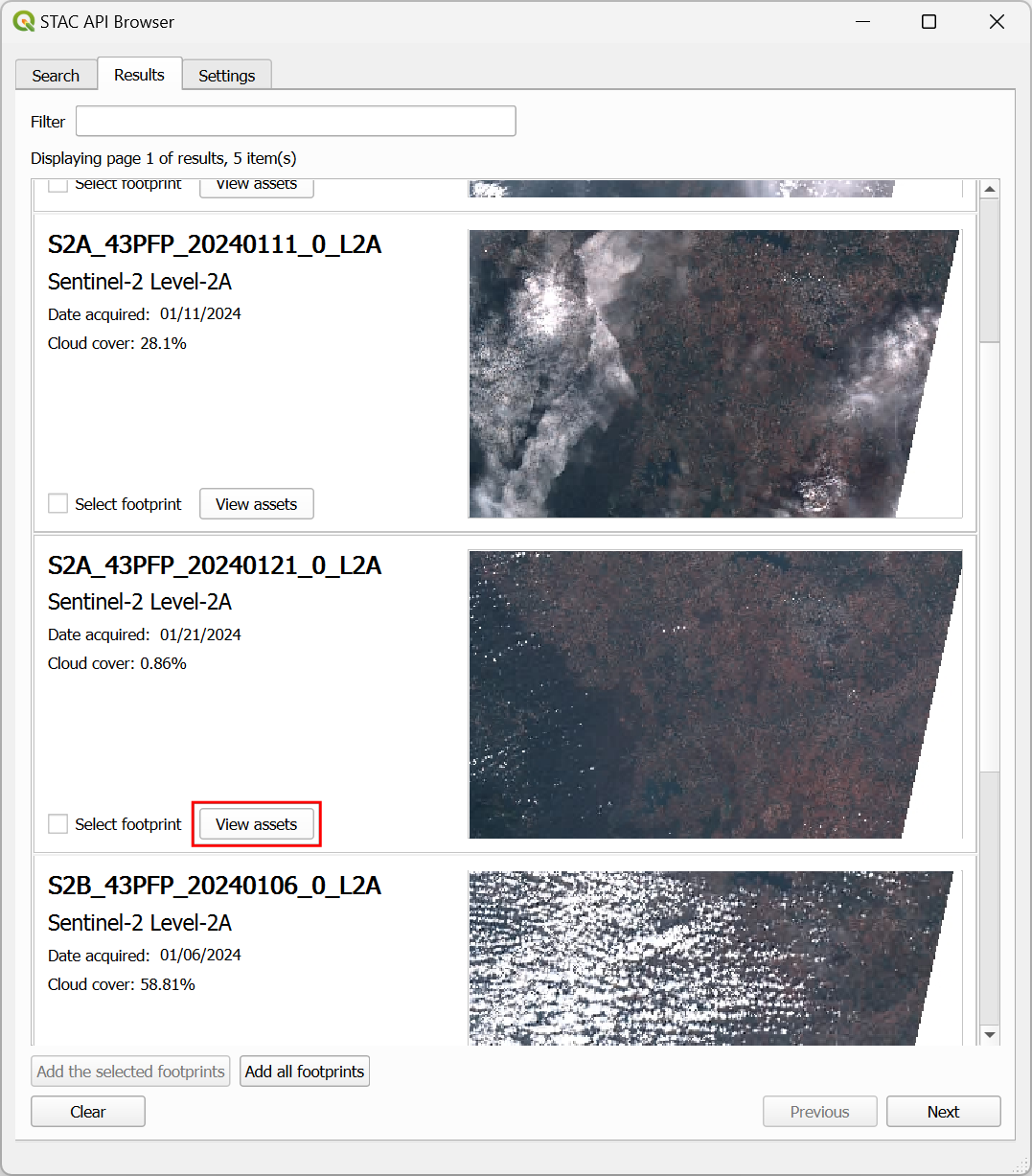
- In the Results tab, you will see the list of matching images. From the preview of the image, locate a reasonably cloud-free image and click View assets.
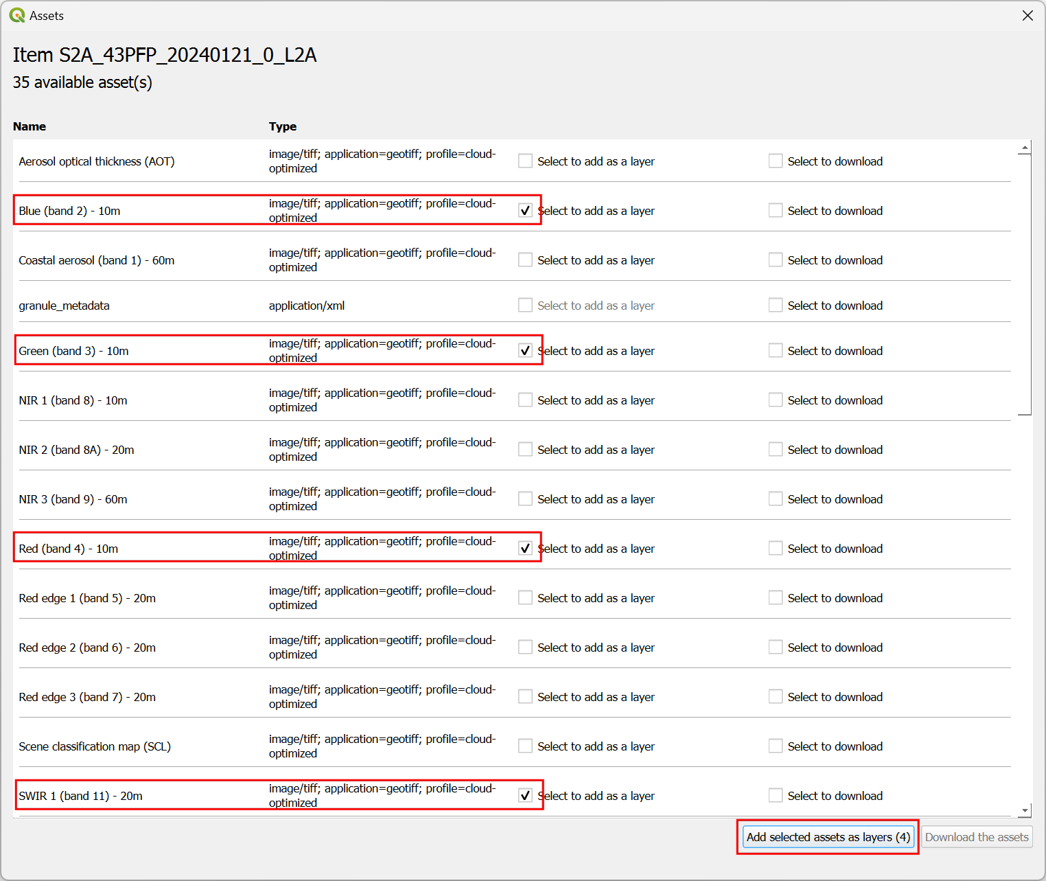
- For this exercise, we will load data for 4 image bands. Check the
Select to add as a layer box for
Blue (band 2),Green (band 3),Red (band 4)andSWIR 1 (band 11). Click Add select assets as layers (4).
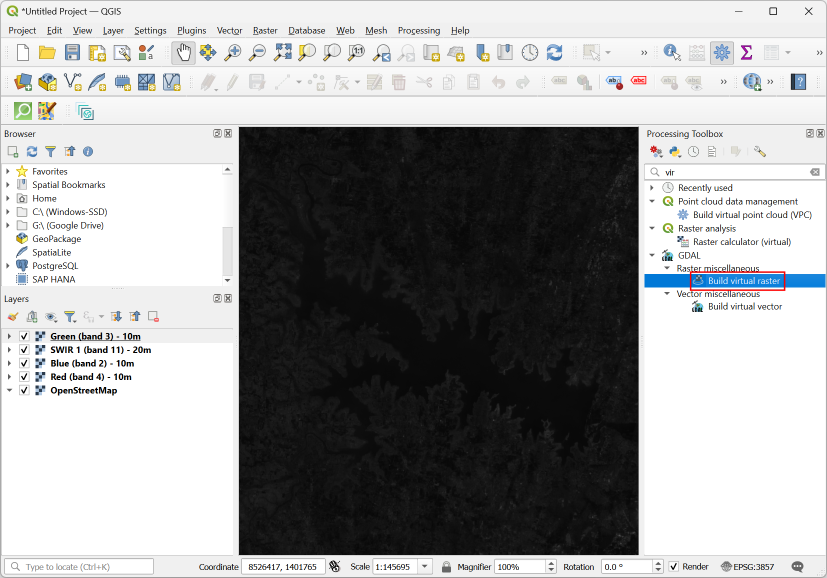
- The selected bands will be loaded as new layers in the main QGIS canvas. Each band is a Cloud-Optimized GeoTIFF (COG) that is hosted on AWS and being streamed to your QGIS. We can combine multiple bands into a single image and visualize it. These are called Color Composites. Let’s stack the Red, Green and Blue bands to create an natural color composite. Go to Processing → Toolbox. From the Processing Toolbox, search and locate the GDAL → Raster miscellaneous → Build virtual raster algorithm. Double-click to open it.
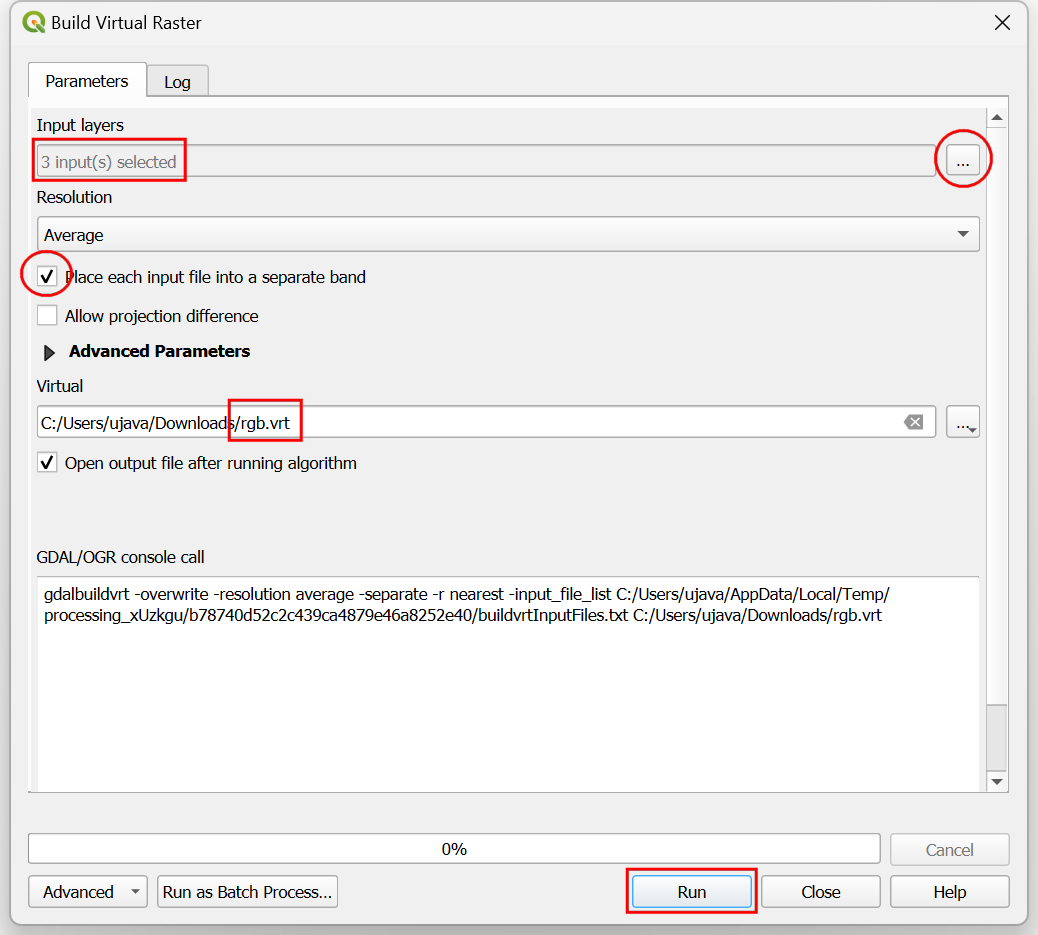
- This algorithm creates a new layer in the Virtual
Raster format which allows you to combine multiple raster layers in
to a single file without consuming extra disk space. Select
Blue (band 2),Green (band 3),Red (band 4)as Input layers and check Place each input file into a separate band. Click the...button next to Virtual and save the output file asrgb.vrt. Next click Run.
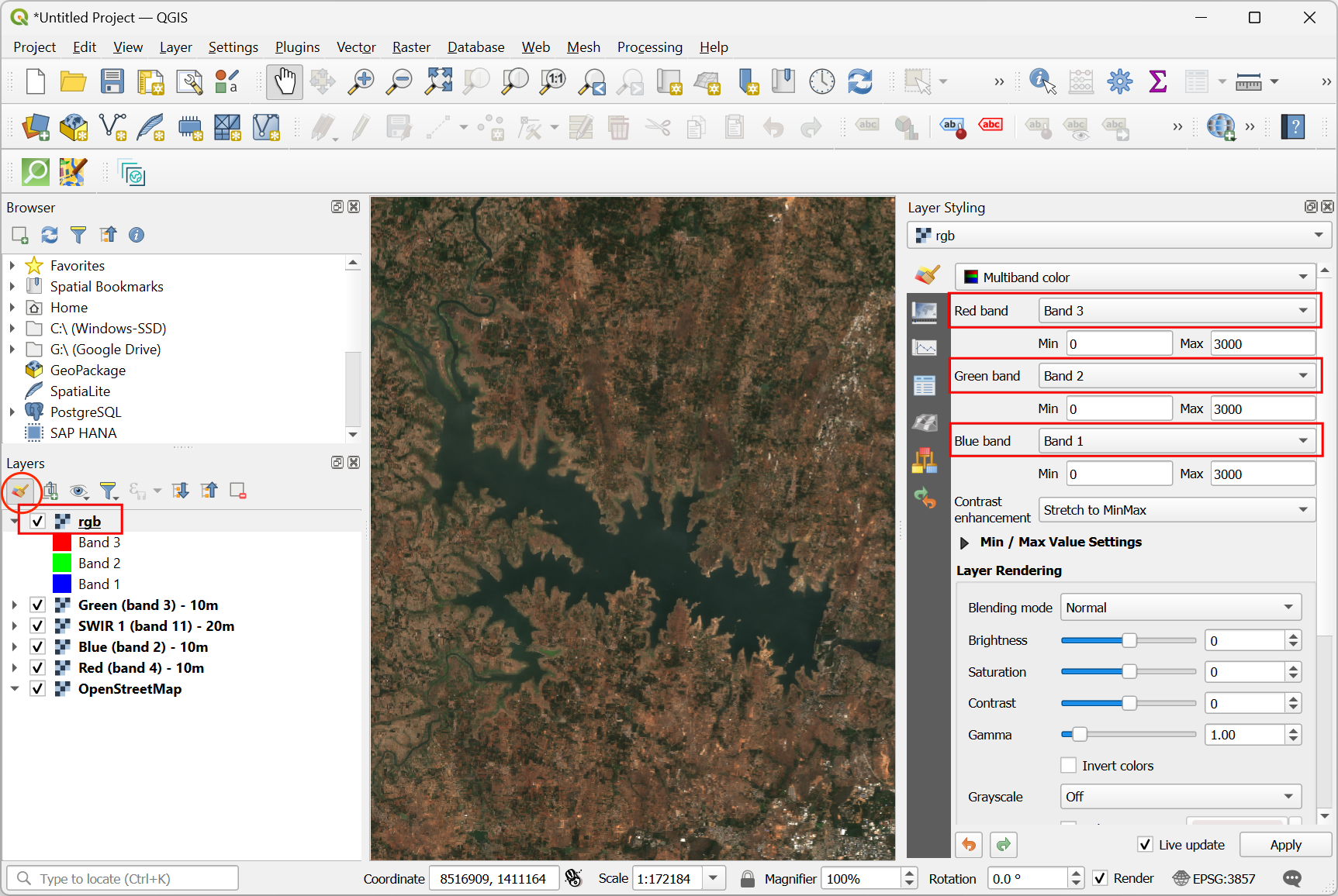
- A new layer
rgbwill be added to the Layers panel. This layer contains references to the 3 different images. Note that the order of the bands in alphabetical, so the mapping in the virtual raster is as follows: Band 1 → Blue (band 2), Band 2 → Green (band 3) and Band 3 → Red (band 4). Open the Layer Styling Panel and placeBand 3,Band 2andBand 1as Red, Green and Blue bands. Change the Min and Max values to0and3000respectively. You will see the image now appear in natural colors.
4.2 Computing a Spectral Index
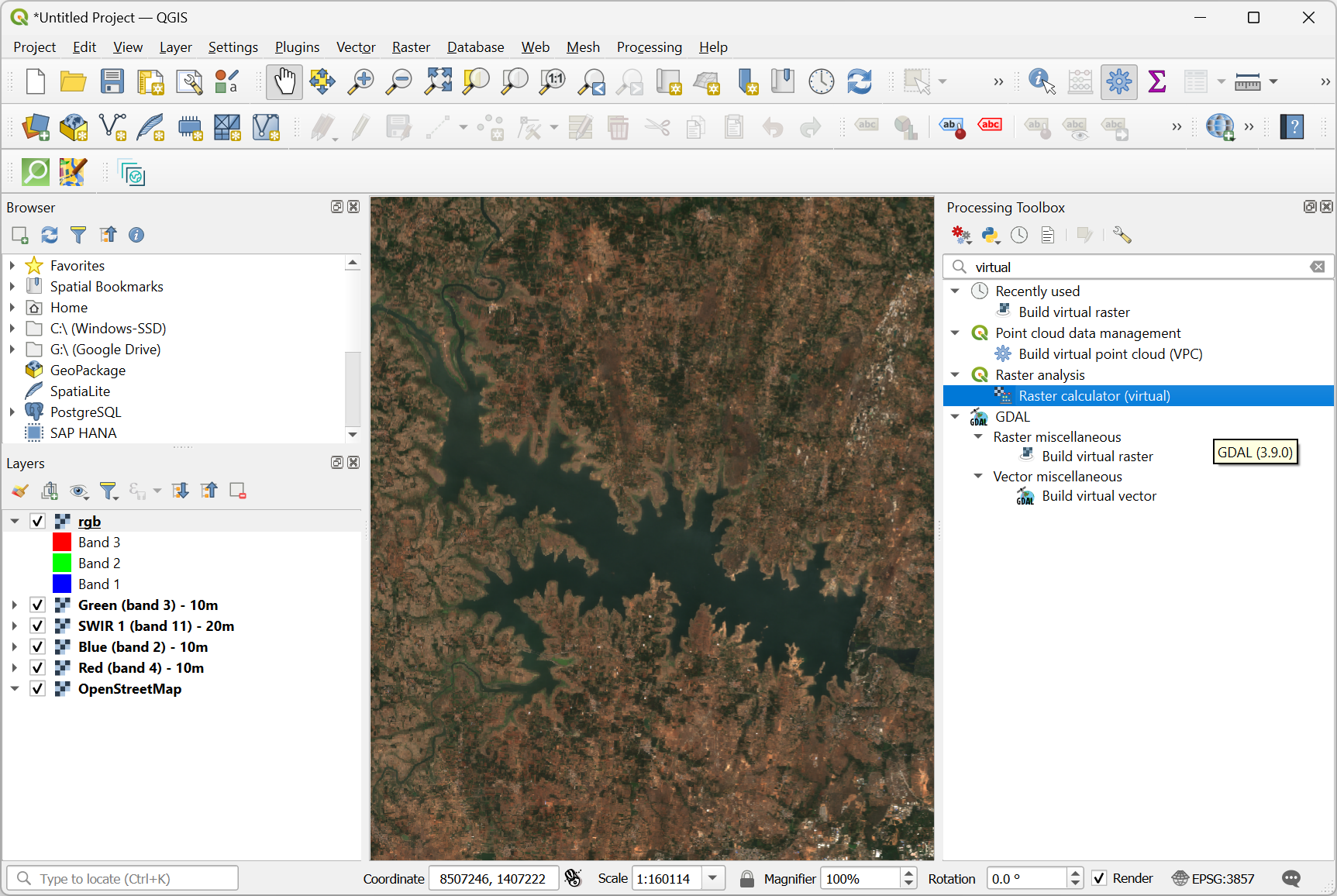
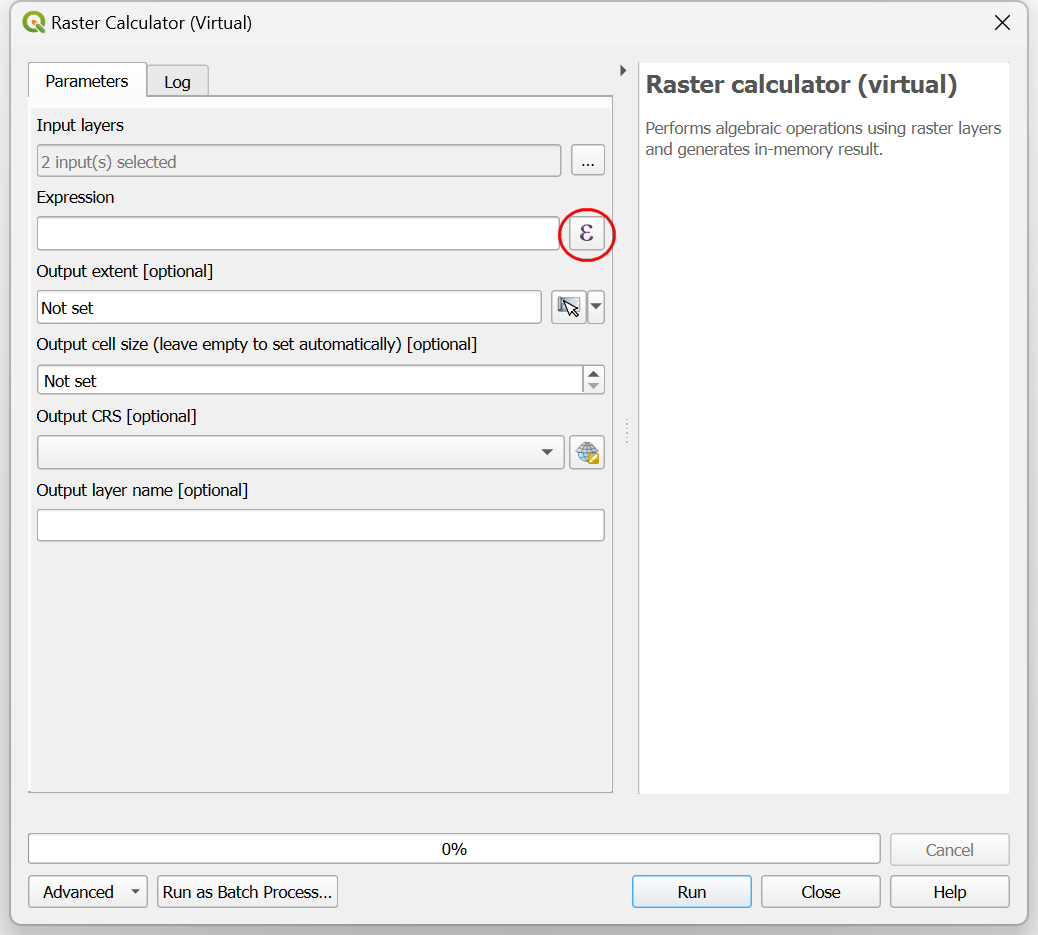
- We can also do some analysis with the satellite image bands. Let’s calculate the Modified Normalized Difference Water Index (MNDWI). This is a widely used spectral index for identifying and extracting water pixels from satellite images. This index is calculated by taking the normalized ratio of the Green (band 3) and the SWIR-1 (band 11) bands. From the Processing Toolbox, search and locate the GDAL → Raster analysis → Raster calculator (virtual) algorithm. Double-click to open it.
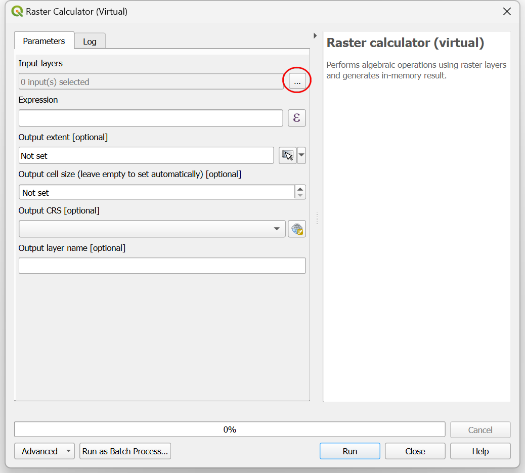
- In the Raster calculator (virtual) dialog, click the
..button for Input layers.
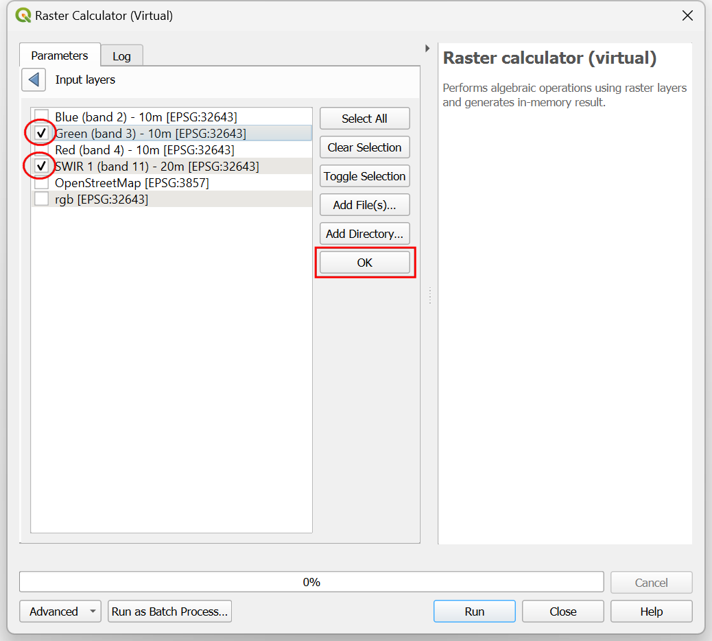
- Select the
Green (band 3)and theSWIR 1 (band 11)layers and click OK.
- Next click the Expression button.
- Remember the formula for MNDWI is (Green - SWIR1)/(Green + SWIR1). You can click on the layer names to enter it in the Raster Calculator Expression and construct the expression as shown below. Once done, click OK.
("Green (band 3) - 10m@1" - "SWIR 1 (band 11) - 10m@1")
/ ("Green (band 3) - 10m@1" + "SWIR 1 (band 11) - 10m@1")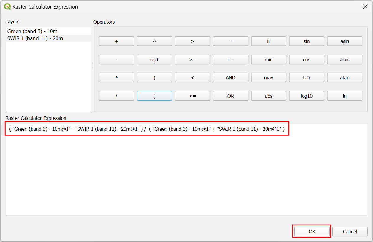
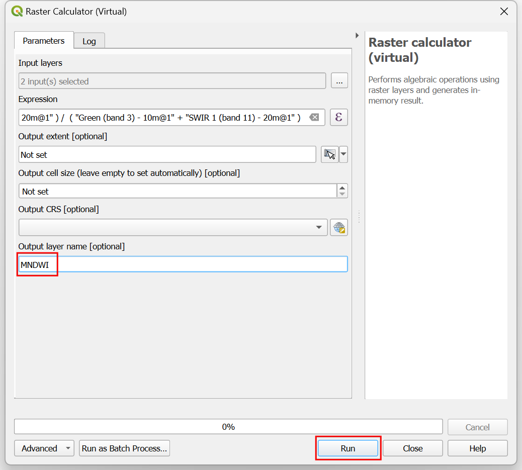
- Enter the Output layer name as
MNDWIand click Run.
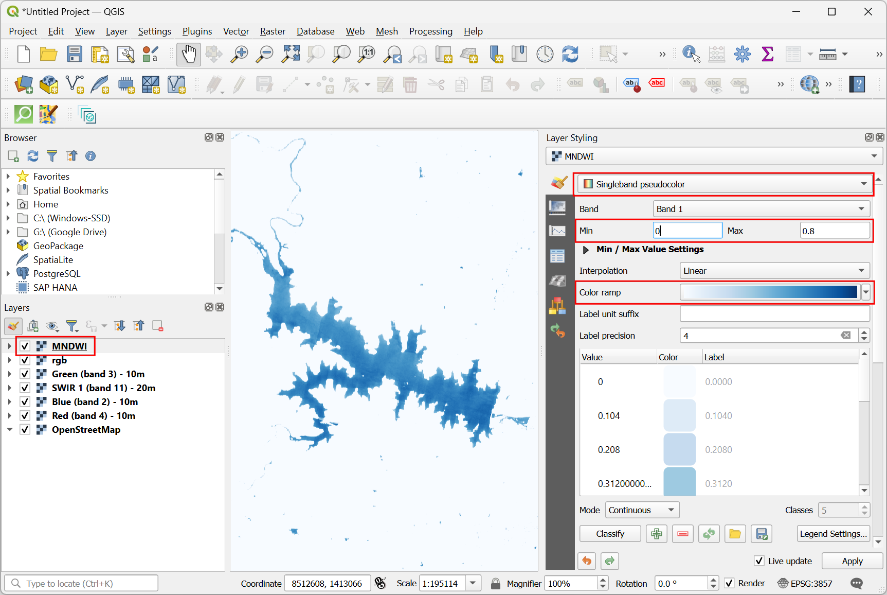
- A new layer
MNDWIwill be added to the Layers panel. Click the open the Layer Styling Panel button. Change the renderer toSingleband psuedocolor. Set the Min and Max values to0and0.8respectively. Choose theBluesas the Color ramp. You will see a visualization where all detected water pixels are highlighted in the blue color.
- The MNDWI image contains values in the range -1 to +1 with pixel values 0 and above typically indicating presence of water. We can extract the water pixels to a new layer by applying a threshold of 0. From the Processing Toolbox, search and locate the GDAL → Raster analysis → Raster calculator (virtual) algorithm. Double-click to open it.
- Select the
MNDWIlayer as the Input layers and enter the expression shown below. Set the Output layer name toWaterand click Run.
"MNDWI@1" > 0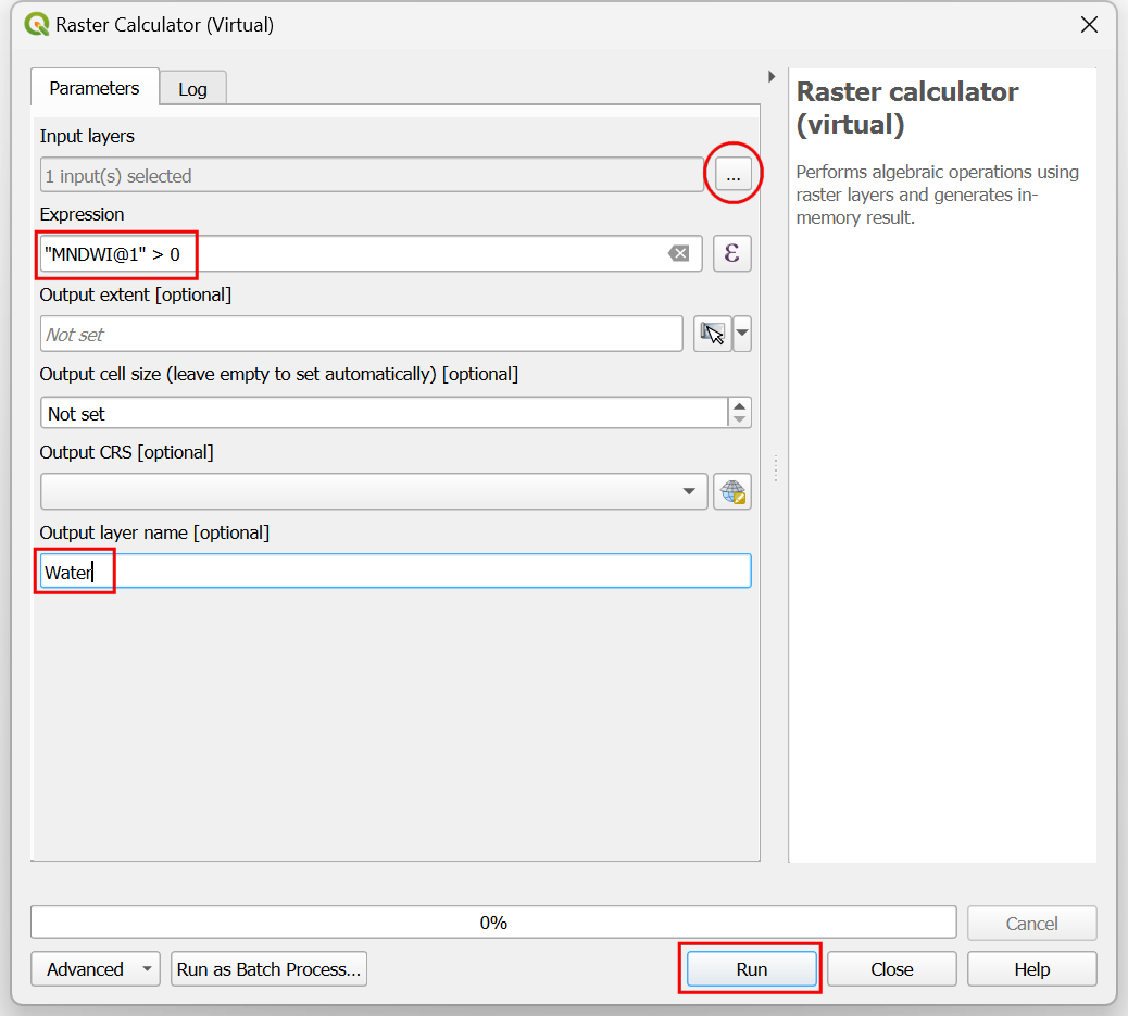
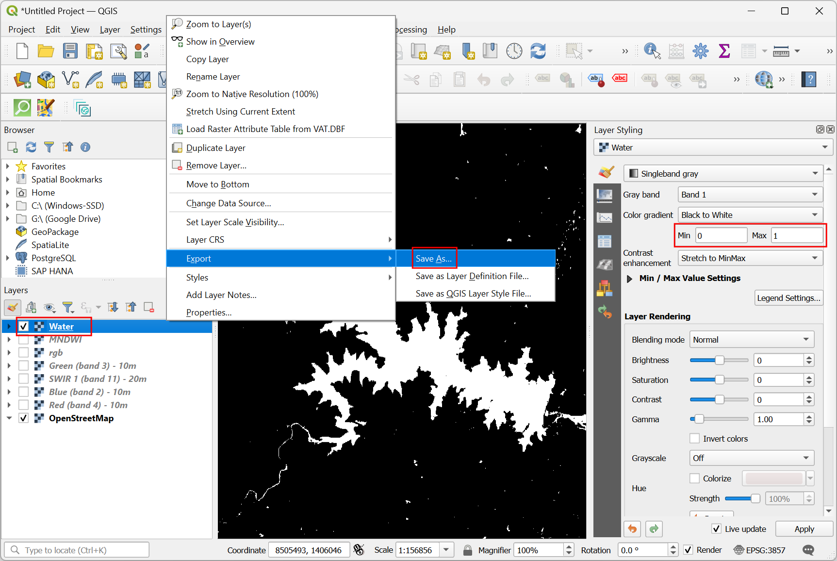
- A new layer named
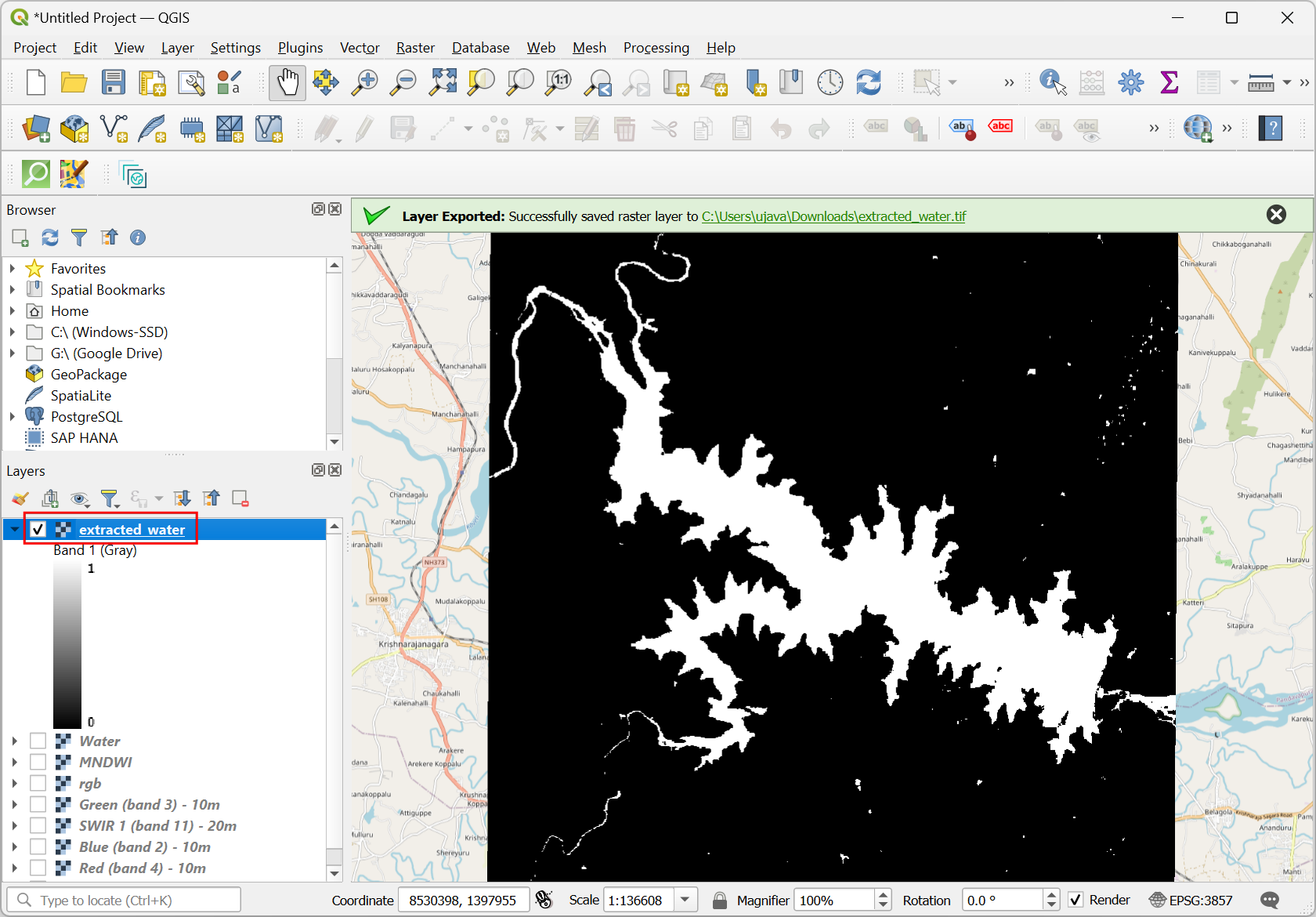
Waterwill be added to the Layers panel. Click the open the Layer Styling Panel button. Set the Min and Max values to0and1respectively. You will see all the extracted water pixels in white. Remember this image is still a virtual image being computed on-the-fly by streaming in the required data directly from the cloud-hosted COGs. You can Zoom and Pan the map and the water pixels will be extracted dynamically. We can save the results as a local GeoTIFF. Right-click on theWaterlayer and select Export → Save As….
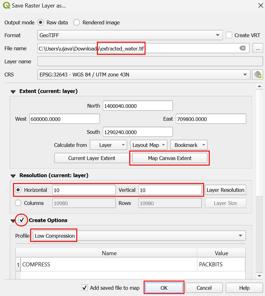
- Click the
..button next to File name and save the file asextracted_water.tif. Expand the Extent section and click the Map Canvas Extent button. Set both both Horizontal and Vertical values for Resolution to be10meters. Check the Create options box and selectLow Compressionas the Profile. Click OK to start the export process. At this stage, QGIS will fetch the required pixels from the cloud dataset at the required resolution, perform the computation to calculate MNDWI and extract the water pixels. Depending on how big is your region, this process may take a few minutes.
- Once complete, a new layer
extracted_waterwill be added to the Layers panel. You were able visualize a satellite image and perform a complex calculation to extract water from the image without first having to download the entire scene. Saving time, bandwidth and computation resources.
Your output should match the contents of the
cloud_native_geospatial_checkpoint4.qgz file in your data
package.
5. Creating and Hosting Cloud Native Geospatial Data
5.1 Creating Cloud Native Geospatial Data
The easiest way to create data in a cloud-optimized format is to use the GDAL/OGR Command-Line Tools. Please check our course material for Mastering GDAL Tools course for step-by-step instructions for installation and usage.
You can use the gdal_translate command to take any
raster data and create a Cloud-Optimized GeoTIFF by specifying the
-of COG option.
gdal_translate -of COG viirs_ntl_2021_global.tif viirs_ntl_2021_global_cog.tifSimilarly, ogr2ogr can convert any supported vector data
format to a cloud-otpmized data format. The command below converts a
GeoPackage to a FGB format using the -f FlatGeobuf
option.
ogr2ogr -f FlatGeobuf hydrorivers.fgb hydrorivers.gpkgYou can create the output dataset by specifying a subset of columns
using the -select option.
ogr2ogr -f FlatGeobuf admin2.fgb admin2.gpkg -select "adm2_name,adm1_name,adm0_name,iso_2,iso_3"5.2 Hosting Cloud Native Geospatial Data
The main advantage of cloud-native data formats is that they can be streamed directly from files, without needing specialized servers. This is achieved by making a HTTP-range request from the file. This means the file needs to be accessible by HTTP as static file objects. Most consumer cloud storage servies such as Google Drive, Microsoft OneDrive, Dropbox etc. do NOT allow direct access to file objects and cannot be used to serve files via HTTP. Below are some recommended options for storing files for cloud-native applications.
Cloud Object Stores
- Google Cloud Storage
- Microsoft Azure Blob Storage
- Amazon S3
- Cloudflare R2
- …
GitHub
- Upload your files to a Github Release (Unlimited free storage for files upto 2GB)
Any Simple HTTP Server
Use any simple HTTP server that can serve static files.
Data Credits
- Global Edge-matched Subnational Boundaries: Humanitarian Edge Matched, FieldMaps, OCHA, geoBoundaries, U.S. Department of State, OpenStreetMap. Downloaded from https://fieldmaps.io/data
- Sentinel-2 Level-2A: Contains Copernicus Sentinel data.
License
This workshop material is licensed under a Creative Commons Attribution 4.0 International (CC BY 4.0). You are free to re-use and adapt the material but are required to give appropriate credit to the original author as below:
Cloud Native Geospatial Workflows with QGIS by Ujaval Gandhi www.spatialthoughts.com
© 2024 Spatial Thoughts www.spatialthoughts.com
If you want to report any issues with this page, please comment below.