From Cloud to Desktop: Working with Earth Engine Data in QGIS (Full workshop)
Unlocking cloud geospatial data with with the Google Earth Engine Plugin for QGIS.
Ujaval Gandhi
![]()
Introduction
Google Earth Engine is a cloud-based platform that enables working with large-scale earth observation datasets effectively. The Google Earth Engine Plugin for QGIS brings this power to the desktop and enables QGIS users to combine their geospatial workflows with cloud-based datasets. This workshop will give you hands-on experience using plugin to leverage cloud-based datasets in desktop-based geospatial workflows.
Installation and Setting up the Environment
Install QGIS
This workshop requires QGIS LTR version 3.44 or above. Please review QGIS-LTR Installation Guide for step-by-step instructions.
Sign-up for Google Earth Engine
If you already have a Google Earth Engine account, you can skip this step.
Visit our GEE Sign-Up Guide for step-by-step instructions.
Install the Google Earth Engine Plugin for QGIS
This workshops requires the Google Earth Engine Plugin for QGIS. The plugin can be installed by the Plugin Manager from the official QGIS plugin repository and involves a few extra steps to authenticate with your Google Earth Engine account and set the Google Cloud project.
Visit the QGIS Earth Engine Plugin Installation Guide for step-by-step instructions.
Get the Data Package
We have created a data package containing checkpoint projects that will allow you to load the results of each section. You can download the data package from qgis-gee-workshop.zip. Once downloaded, unzip the contents to a folder on your computer.
Get the Workshop Video
The workshop is accompanied by a video covering the all the sections. This video is recorded from our live online class and is edited to make them easier to consume for self-study. We have 2 versions of the videos:
YouTube
The video on YouTube is ideal for online learning and sharing. You may also turn on Subtitles/closed-captions and adjust the playback speed to suit your preference. Access the YouTube Video ↗
Vimeo
We have also made full-length video available on Vimeo. This video can be downloaded for offline learning. Access the Vimeo Video ↗
Overview of the Earth Engine Data Model
Earth Engine supported georeferenced raster and vector datasets. The terminology used by Earth Engine is different than used by QGIS. Below is the explanation of common data types in Earth Engine.
- Image: A single georeferenced raster dataset. It can have one or more bands. The image metadata is stored as properties. Each band in the image can have different data type, spatial resolution (i.e. scale) and projection.
- ImageCollection: The most common type of dataset used in Earth Engine that consists of multiple Image objects. Images over both space and time can be put in a single ImageCollection.
- FeatureCollection: Vector datasets are represented as FeatureCollections in Earth Engine. Each Feature in the collection consists of a geometry and some properties.
Accessing Earth Engine Datasets
Official Data Catalog
The Google Earth Engine team maintains a large catalog of ready-to-use datasets that can be readily accessed via the plugin. You can search and browse the datasets at the Earth Engine Data Catalog.

Awesome GEE Community Catalog
The Earth Engine Community, led by Samapriya Roy maintains another large catalog of datasets that have been processed and ingested in Earth Engine. This catalog can be accessed from awesome-gee-community-catalog. The dataset available in this catalog can also be used directly in the QGIS Earth Engine plugin.

User-Uploaded Assets
Earth Engine users can also upload their own datasets and use them in the plugin. This is useful if you wanted to access your private assets through the QGIS Earth Engine plugin. You must be either the owner of the asset or need read access to the asset.
Hands-on With QGIS Earth Engine Plugin
1. Downloading Images from Earth Engine
The Google Earth Engine plugin comes with a handy Export Image to GeoTIFF algorithm that allows you to download images from GEE directly to your computer as GeoTIFF files. In this tutorial, we will use the plugin to create a Sentinel-2 median composite for a region and download it as a GeoTIFF file.
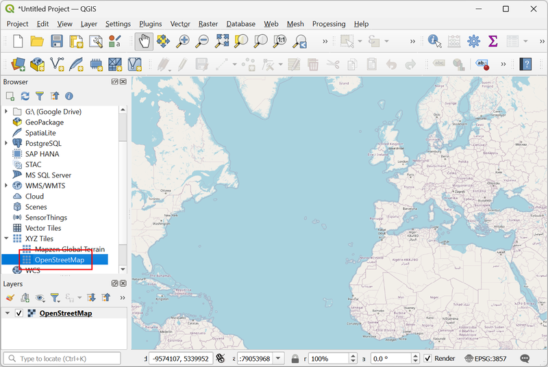
- Open QGIS. To help us select a region of interest, it will be helpful to have a basemap. From the QGIS Browser Panel, locate the XYZ Tiles → OpenStreetMap layer and drag it to the canvas.
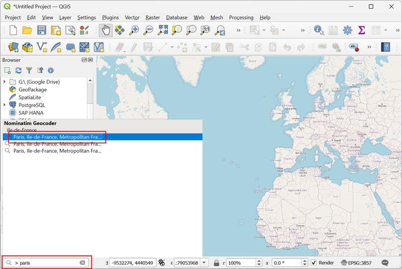
- We can use the QGIS’s built-in geocoder to search for a place. For
this tutorial, we want to download imagery over Paris. Select the
locator bar in the bottom left corner and enter the search term
> paris. Make sure there is a space between the>character and the search term. From the results, click on the first one to zoom to the location.
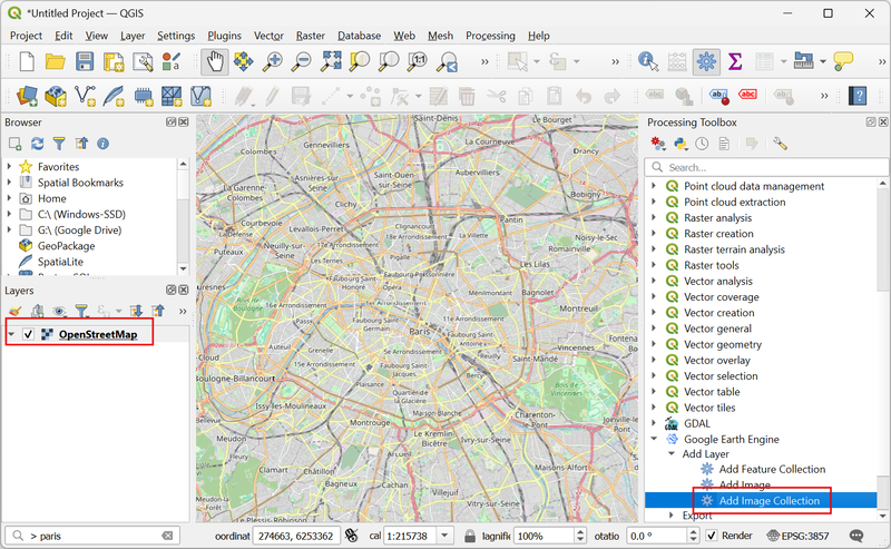
- Zoom and pan the map to the desired extent. Open the Processing Toolbox from Processing → Toolbox. Locate the Add Image Collection algorithm from the Google Earth Engine provider. Double-click to open it.
- To add an Image Collection, we first need to find the Image Collection ID for the Sentinel-2 Level-2A collection.
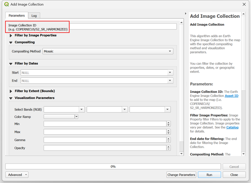
- Open the Earth Engine
Data Catalog and navigate to the dataset page for Harmonized
Sentinel-2 MSI: MultiSpectral Instrument, Level-2A (SR). Copy the
Image Collection ID
COPERNICUS/S2_SR_HARMONIZEDshown on the page.

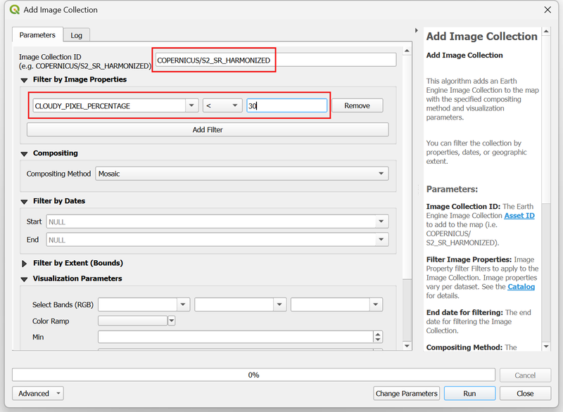
- Back in the Add Image Collection dialog, paste the Image
Collection ID
COPERNICUS/S2_SR_HARMONIZED. Next, we can apply a metadata filter to select images with less cloud. In the Filter by Image Properties section, selectCLOUDY_PIXEL_PERCENTAGEas the property,<as the operator and enter30as the value. This will select all images with < 30% cloud cover.
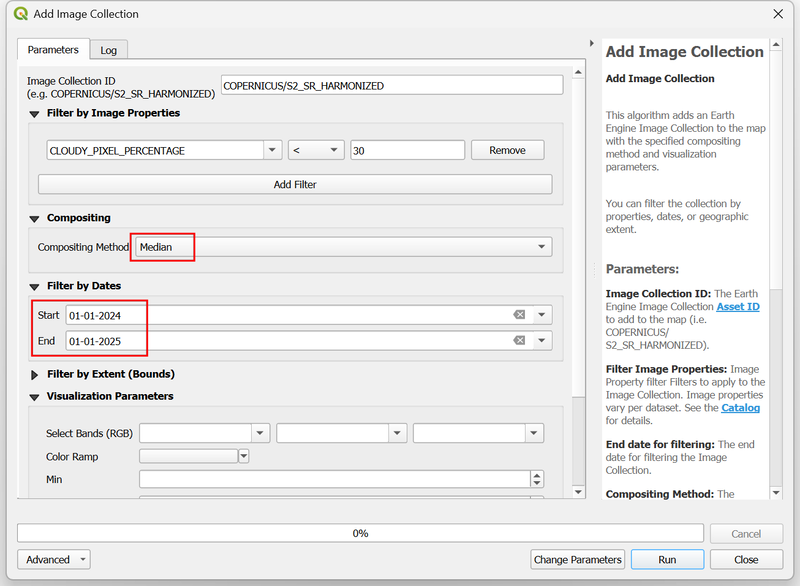
In the Compositing section, select
Medianas the Compositing Method. This method will take all available images and calculate the median value for each pixel. For optical imagery, such as Sentinel-2, this method is useful in selecting the best representative pixel for the chosen duration without being affected by outliers such as clouds and cloud-shadow. We want to create an annual composite, so in the Filter by Dates section, enter the Start and End dates as01-01-2024and01-01-2025.Remember that the End date in the Earth Engine date filter is exclusive - so we need to add an extra day to ensure do not exclude the last day of the year.
- Expand the Filter by Extent (Bounds) section. Click the
Map Canvas Extentbutton to load the selected region in the canvas.

- Before loading the image, we need to specify the visualization
parameters. For multi-band images, we can select 3 bands to be used for
visualization. We will visualize the resulting image in natural color,
so select
B4(Red) ,B3(Green) andB2(Blue) as the bands. The typical range of pixel values for Sentinel-2 images are between 0-3000, so enter0as Min and3000as Max. Check the Clip to Extent box to load only the pixels within the selected extent and click Run.

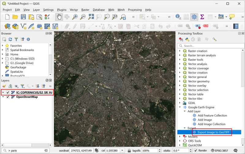
- Once the algorithm finishes, a new layer
IC: COPERNICUS/S2_SR_HARMONIZED (Median)will be added to the Layers panel. This layer is being streamed from the Earth Engine servers. As you zoom or pan the image - new pixels will be computed on-the-fly and displayed. Lets download this image so we can use it within QGIS for analysis. Locate theExport → Export Image to GeoTIFFalgorithm from the Google Earth Engine provider in the Processing Toolbox. Double-click to open it.
If the image appears blank, move the map slightly using the Pan tool. This will refresh the canvas and request loading of the tiles from Earth Engine.
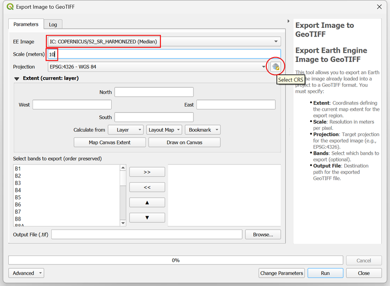
- In the Export Image to GeoTIFF dialog, select
IC: COPERNICUS/S2_SR_HARMONIZED (Median)as the EE Image. We want to export this at its native resolution, so enter10as the Scale (meters). We can also specify the projection in which we want the output image. Click the Select CRS button.
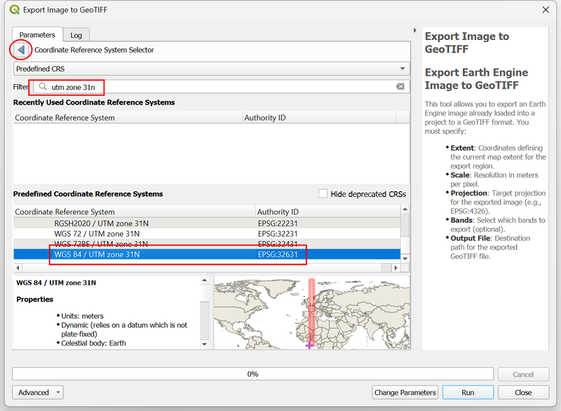
- It is recommended to use a Projected CRS suitable for the region of
interest. UTM is a good choice for such a CRS. We can find the CRS for
the UTM Zone where our region is located. If you do not know the UTM
Zone, you can use this handy What
UTM Zone am I in? map. Paris is located in the UTM Zone
31N. Search and select the
WGS84 / UTM zone 31N (EPSG:32631)CRS. Once selected, click the arrow at the top of the selector to go back to the previous dialog.
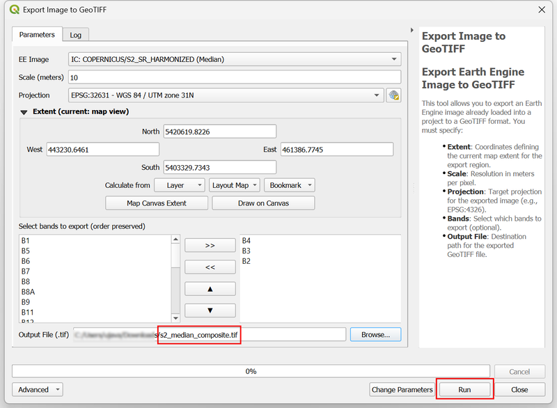
- Next, select the Map Canvas Extent as the Extent of the image for Export. We can choose the subset and order of bands to export. For this tutorial, lets export the B4, B3 and B2 bands. You can select each band from the left-hand section and use the >> button to add them to the list of output bands.

- For the Output File, browse to a directory on your computer
and enter the file name as
s2_median_composite.tif. Once configured, click Run.
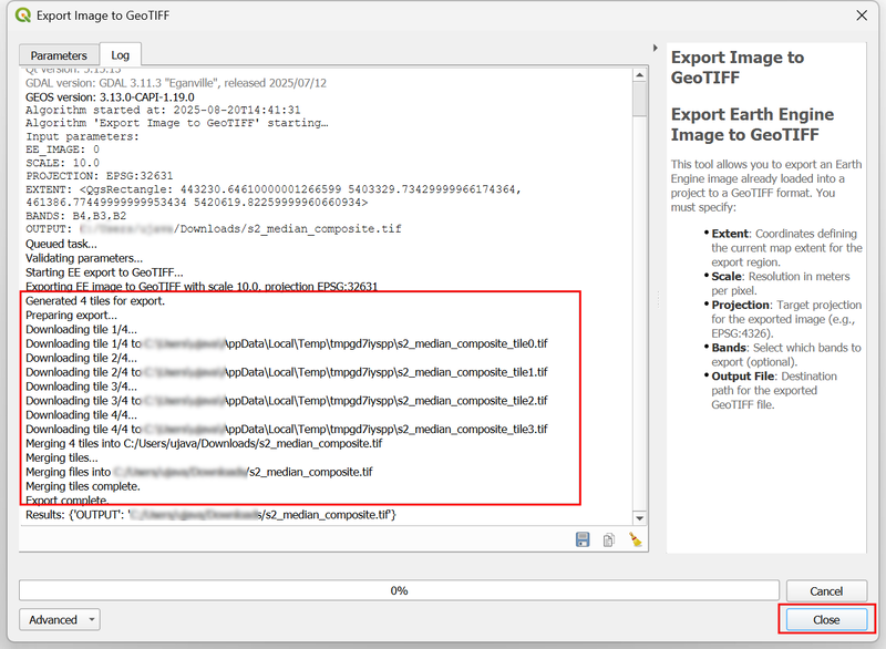
- The requested region will be divided into smaller tiles and each tile will be downloaded separately. The algorithm will then merge the downloaded tiles into a single mosaic and save it at the requested location. Depending on the size of the region, resolution, number of bands, and your internet bandwidth, this process can take some time. Once the algorithm finishes, click Close.
- In the layer panel, turn off the
IC: COPERNICUS/S2_SR_HARMONIZED (Median)layer as it is no longer required. In the Browser panel, locate the directory where you saved the output file. Drag and drop thes2_median_composite.tiffile to the canvas to see the downloaded image.

2. Building Workflows with Model Designer
The processing algorithms provided by the Google Earth Engine plugin can be used in the QGIS Model Designer to automate workflows that combine data from the Earth Engine Data Catalog with processing algorithms from QGIS.
In this section, we will build a model that will run the following steps in a single workflow:
- Load landcover data from the Earth Engine Data Catalog
- Download the data as a GeoTIFF file for the chosen region
- Calculate area of each landcover class
- Convert the computed area to square kilometers
- Add input validation to the model
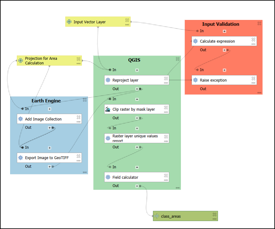
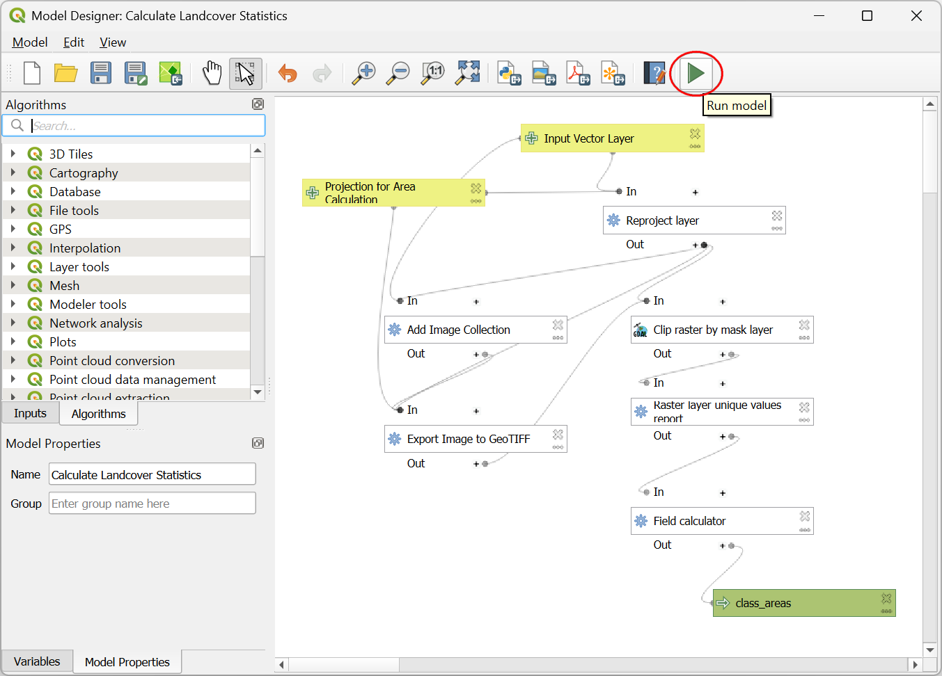
QGIS Model for Calculating Landcover Statistics
There are many landcover datasets available in the Earth Engine Data Catalog as well as GEE Community Catalog. A similar process can be used to load any of the available datasets.
We will use the ESA WorldCover 10m v200 global land cover map for 2021 at 10 m resolution. Visit the dataset description page and note the ImageCollection ID.

This dataset contains a data band named Map and 11-class classification with each class assigned a value between 10-100.

2.1 Building the model
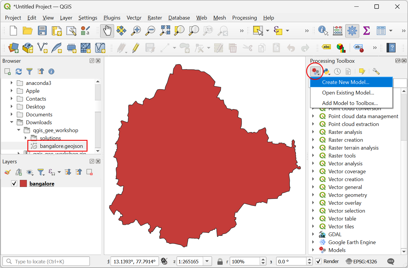
- Open QGIS. From the QGIS Browser Panel, locate the supplied
bangalore.geojsonfile and double-click to open it. This will load a vector layer containing a single feature representing the municipal boundary for the city of Bengaluru, India. Next, open the Processing Toolbox from Processing → Toolbox. From the toolbar, select Models → Create New Model...
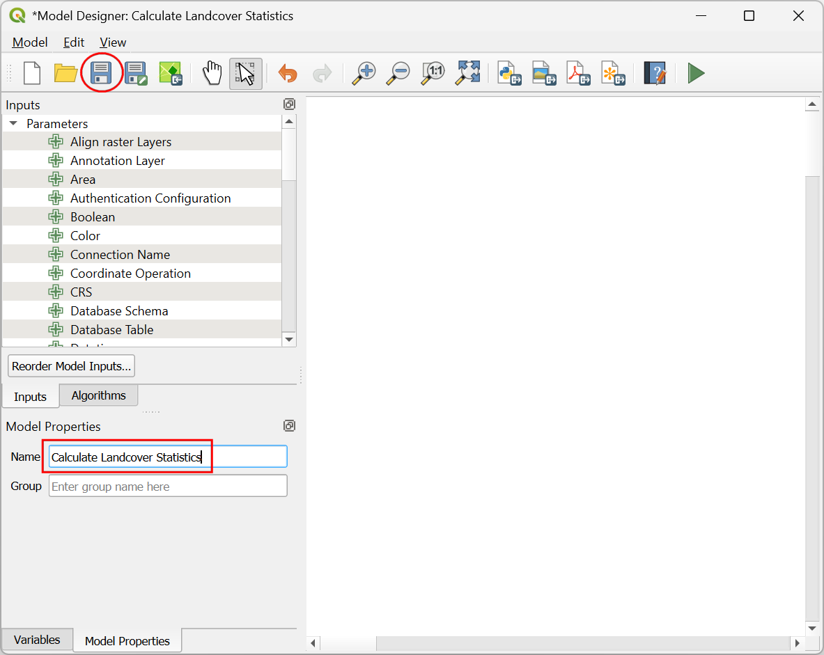
- In the Model Designer dialog, enter the model Name as
Calculate Landcover Statisticsand click the Save model button. When prompted to enter the file name, entercalculate_landcover_statistics.model3.
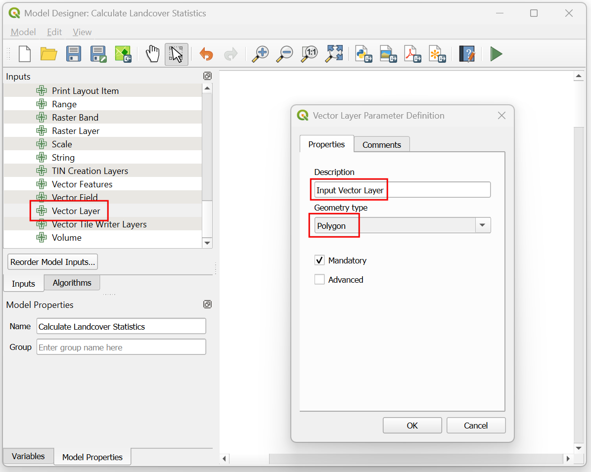
- We will now start building the model. The first input to the model
will be the layer with region boundary. From the Inputs tab,
scroll down to find the + Vector Layer input. Drag it to the
canvas. In the Vector Layer Parameter Definition dialog, enter
Input Vector Layeras the Description and selectPolygonas the Geometry type. Click OK.
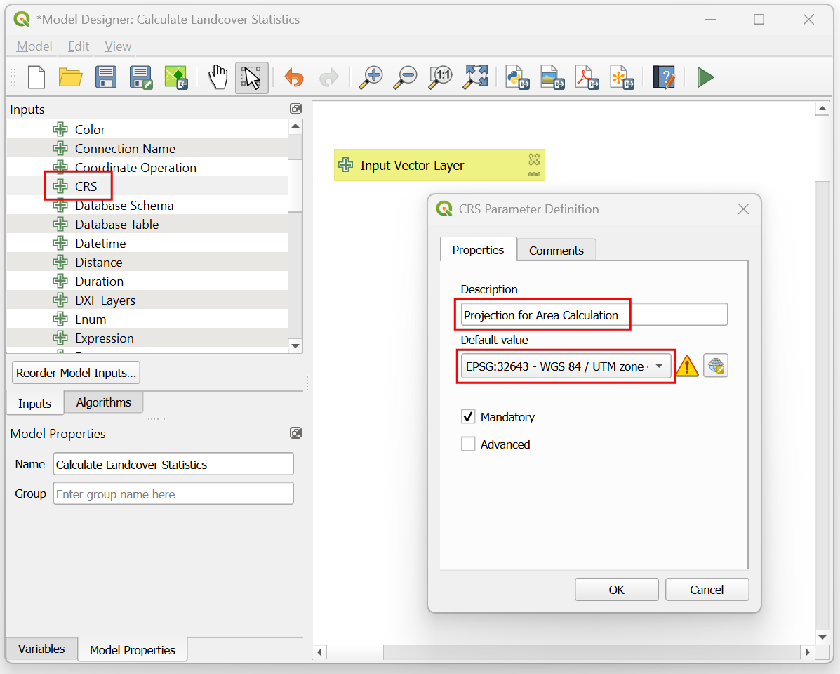
- Next we will add an input for the user to specify the CRS to be used
for the analysis. Locate the + CRS input and drag it to the
canvas. In the CRS Parameter Definition dialog, enter
Projection for Area Calculationas the Description. As the layer we are using falls in the UTM Zone 43N, we can enter the Default value of the CRS asEPSG:32643 - WGS84 / UTM Zone 43N. Click OK.
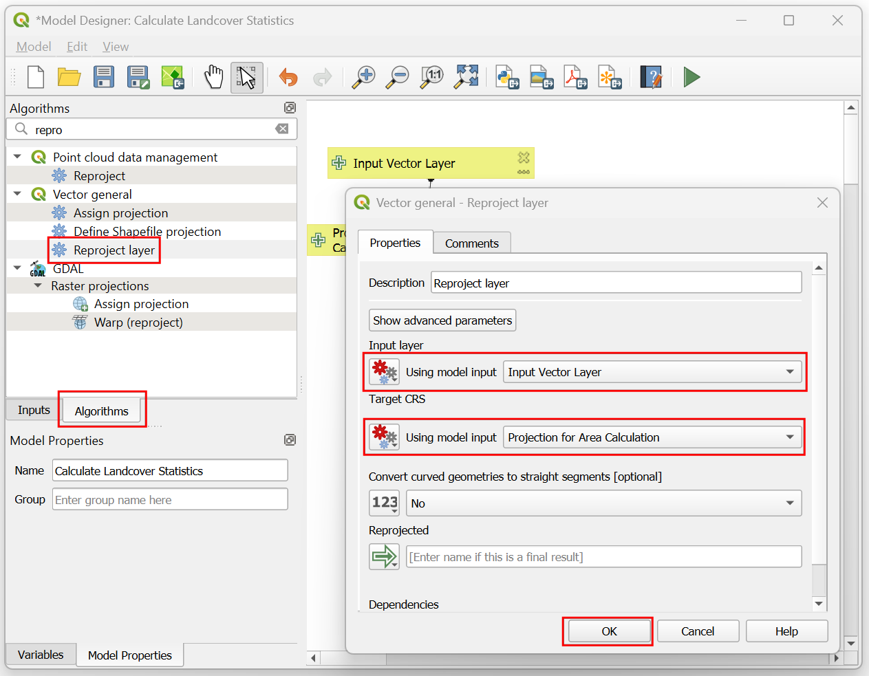
- Once the inputs are configured, lets start building the workflow.
First step is to reproject the input layer to the specified CRS. Switch
to the Algorithms tab, search and locate the Vector general
→ Reproject layer algorithm and drag it to the canvas. In the
Vector general - Reproject layer dialog, switch to Using
model input for Input layer and select the
Input Vector Layerparameter. Similarly for Target CRS select theProjection for Area Calculationparameter. Click OK.
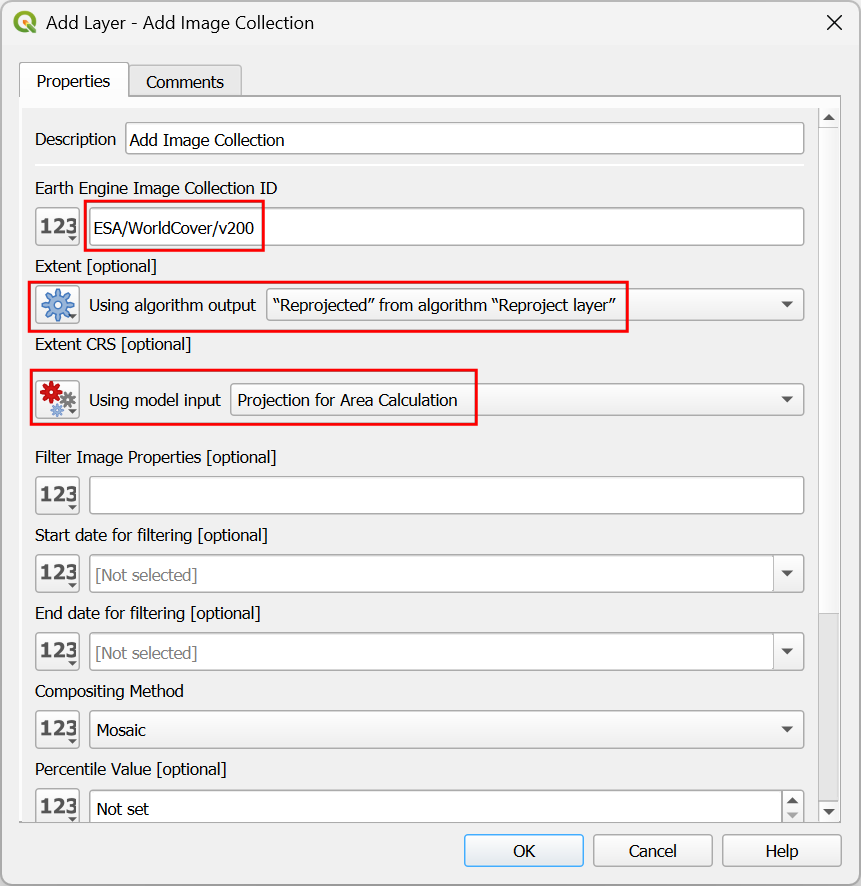
- Next step is to load the dataset from Earth Engine. Scroll down to the Google Earth Engine provider and locate the Add Image Collection algorithm. Drag it to the canvas.

- Enter the Earth Engine Image Collection ID
ESA/WorldCover/v200for the ESA WorldCover dataset. For the Extent, switch to Using algorithm output and select"Reprojected" from algorithm "Reproject layer". For the Extent CRS, select Using model input and selectProjection for Area Calculation.
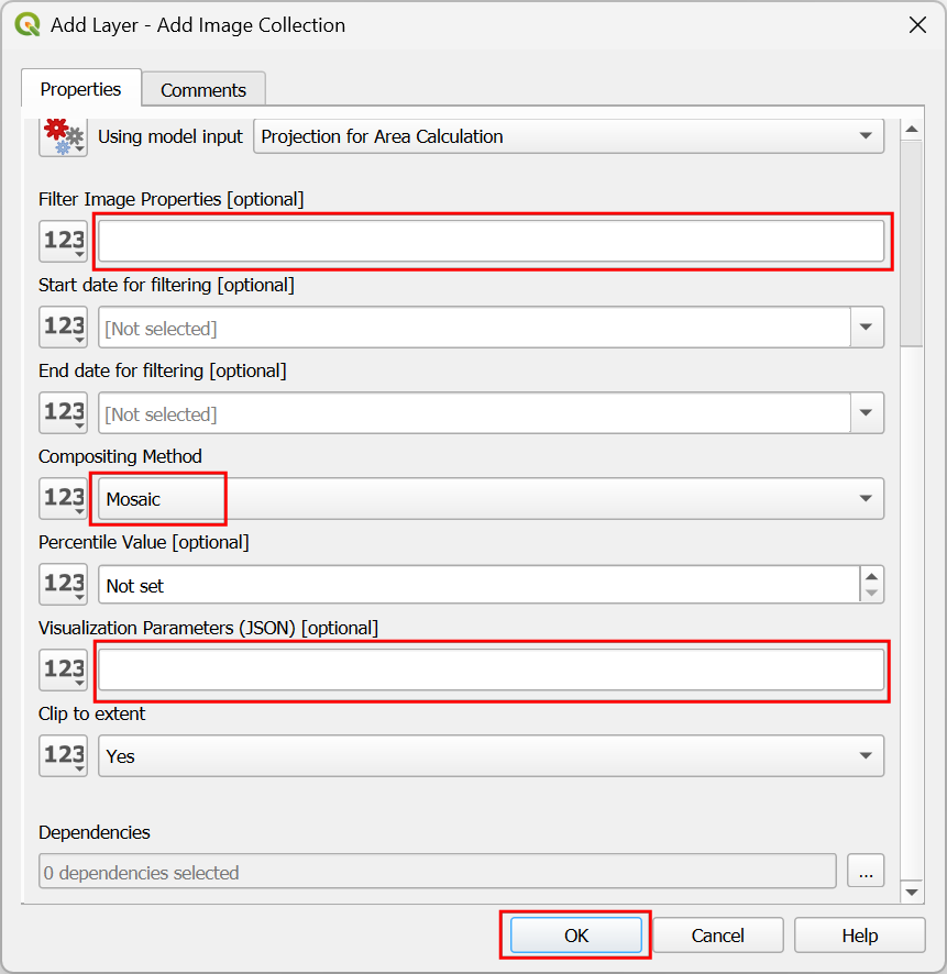
- Scroll down in the dialog and delete the default help text for both
Filter Image Properties and Visualization Parameters
(JSON). Select
Mosaicfor the Compositing Method and click OK.
- The next step is to connect the Export Image to GeoTIFF algorithm. Locate it and drag it to the canvas.
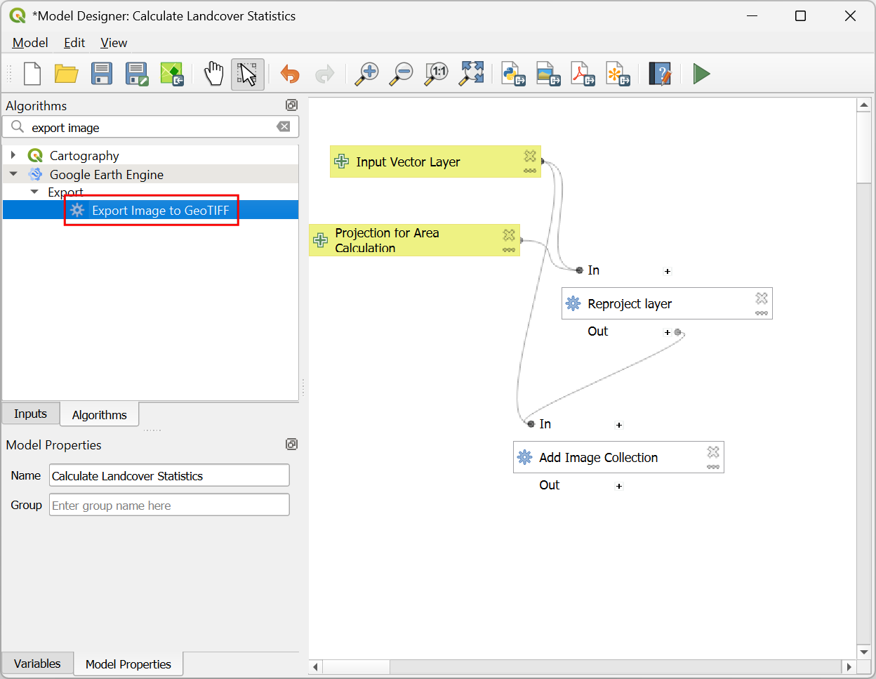
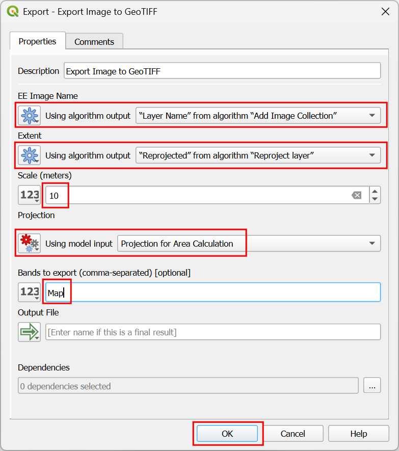
- In the Export Image to GeoTIFF dialog box, for the EE
Image Name, switch to Using algorithm output and select
"Layer Name"from algorithm "Add Image Collection". For Extent, switch to Using algorithm output and select"Reprojected" from algorithm "Reproject layer". The spatial resolution of the dataset is 10m, so enter10as the Scale (meters). EnterMapas the Bands to export. Click OK.
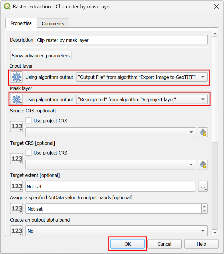
- The previous step will download the data for the given extent as a GeoTIFF file. Let’s clip this to the area of interest. Search and locate the GDAL → Raster extraction → Clip raster by mask layer algorithm and drag it to the canvas.

- In the Raster extraction - Clip raster by mask layer
dialog, configure the Input layer by switching to Using
algorithm output and selecting
"Output File" from algorithm "Export Image to GeoTIFF". Specify the Mask layer by switching to Using algorithm output and selecting"Reprojected" from algorithm "Reproject layer". Click OK.
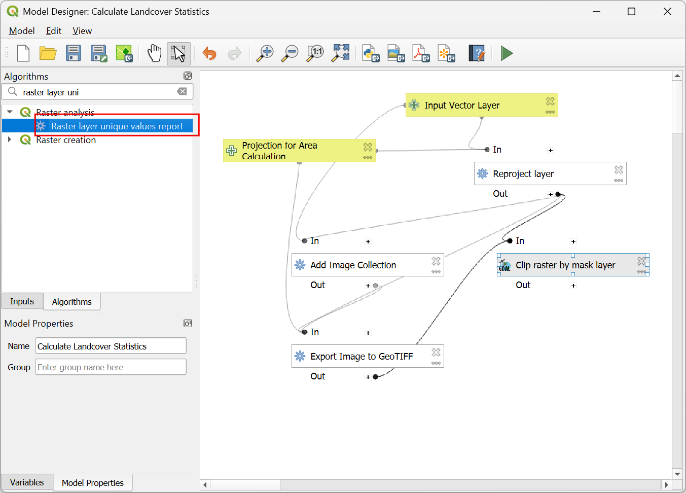
- Now we will add a step to calculate the area for each class. This is done using the Raster analysis → Raster layer unique values report algorithm. Locate it and drag it to the canvas.
Note: The Raster layer unique values report algorithm gives you the areas for the entire raster layer. If you want to calculate areas for different regions over the raster, you can use the Zonal histogram tool to get pixel counts for each class and then multiply it with the area of each pixel.
- In the Raster analysis - Raster layer unique values report,
configure the Input layer by switching to Using algorithm
output and selecting
"Clipped (mask)" from algorithm "Clip raster by mask layer". Keep other parameter values to their default and click OK.

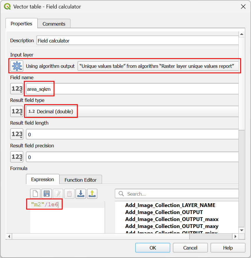
- The results from the previous step will be a table with columns value and m2 containing the class value and total area in square meters. Let’s convert the area to square kilometers. Locate the Vector table → Field calculator algorithm and drag it to the canvas.

- In the Vector table - Field Calculator dialog, configure
the Input layer by switching to Using algorithm output
and selecting
"Unique values table" from algorithm "Raster layer unique values report". Enter the Field name asarea_sqkmand Result field type asDecimal (double). For the Formula, we will divide the area in square meters by 1000 x 1000 (i.e. 1e6) to convert it to square kilometers. Enter the expression as"m2"/1e6.
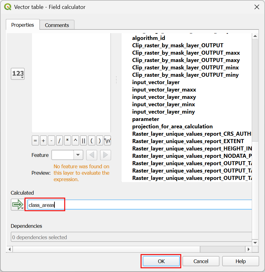
- As this table will be our final output, enter the Calculate
layer name as
class_areasand click OK.
- The model is now complete. Click the Run model button.
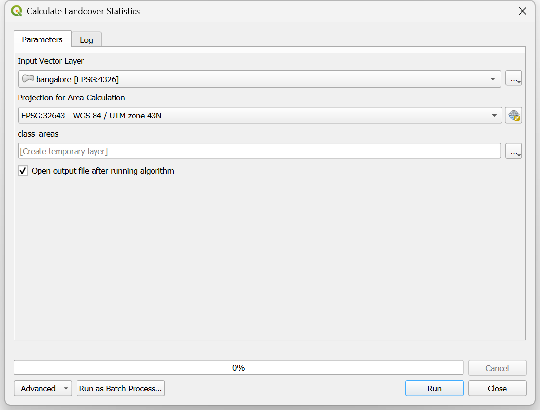
- In the Calculate Landcover Statistics, select
bangaloreas the Input Vector Layer. Keep the other values to their default and click Run.
- Once the model run completes, a new layer
class_areaswill be added to the Layers panel. Open the attribute table and you will see new column with class area statistics computed from the ESA WorldCover dataset..

- It is a good practice to save the model along with the QGIS project so it is always available to whoever is using the project file. Click the Save model in project button to embed the model in your QGIS project file.

- From the main QGIS interface, you will now see a new folder Project models in the Processing Toolbox containing the model we created.

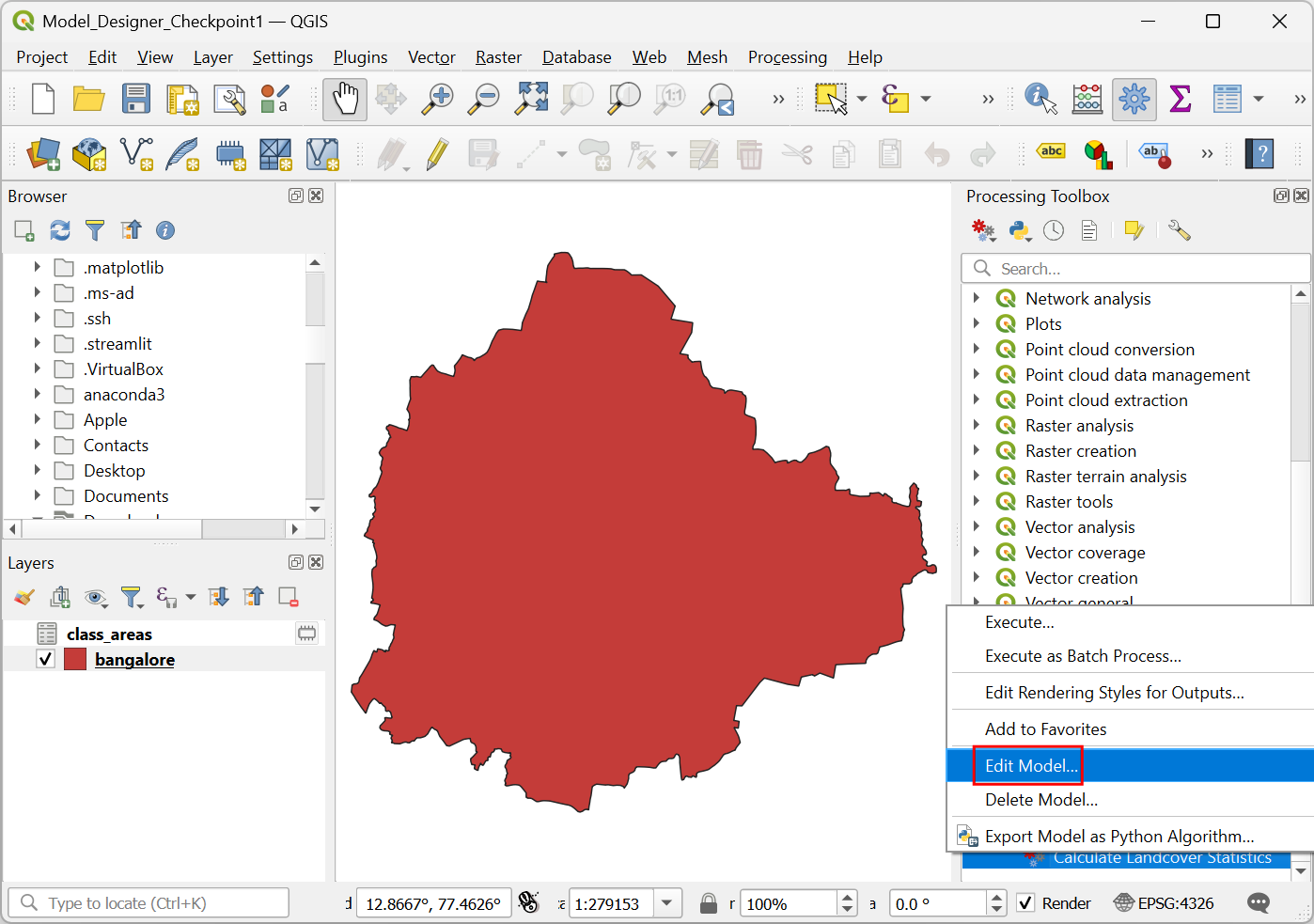
If you’d like to catch up to this point, you can load the
Model_Designer_Checkpoint1.qgz file in the
solutions folder of the data package.
2.2 Validation and Organization
At this point, the model works and generates the landcover statistics for any input region in the world. Let’s learn how to get the model production ready by adding some validation checks and adding visual cues to make model maintenance easy.
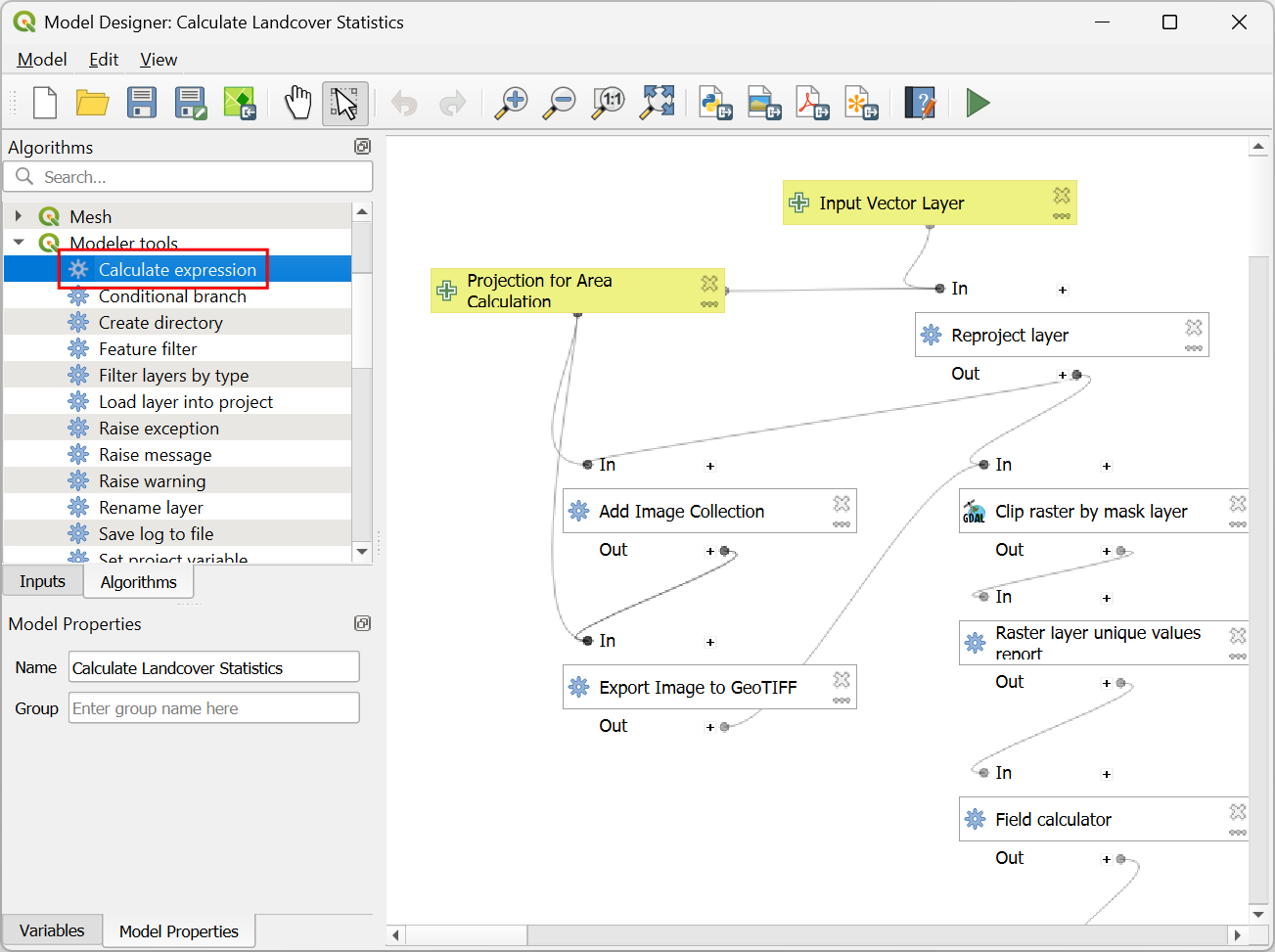
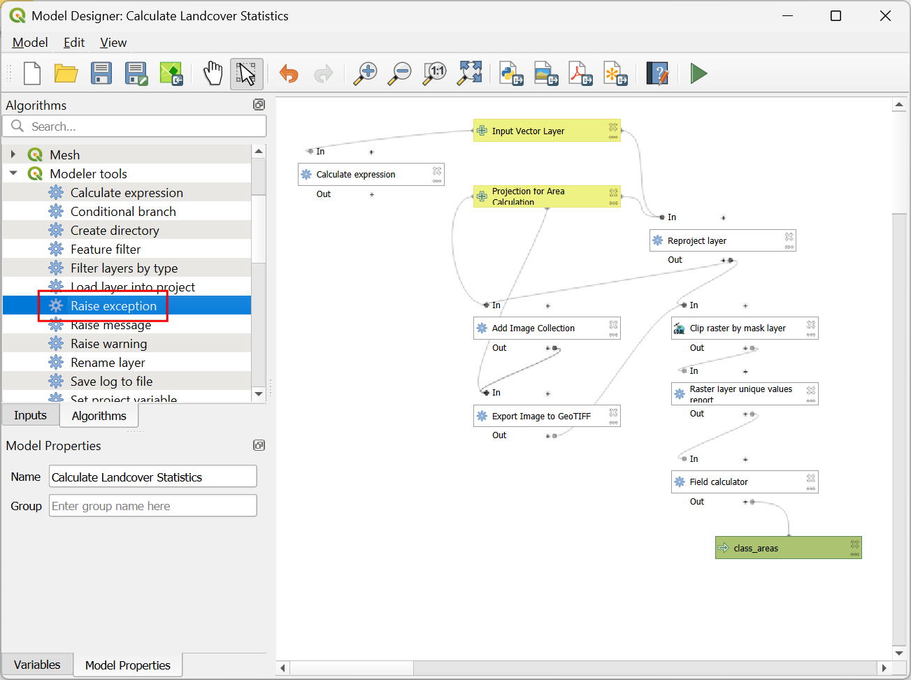
- The model is saved in the Processing Toolbox in the Project models folder. Select the Calculate Landcover Statistics model, right-click and select Edit Model….
- Our input vector layer is expected to have only a single polygon in it. The model does not work with vector layers containing more than 1 polygon. To ensure the supplied layer meets this criteria, we will add a check and raise an error if the feature count of the layer is more than 1. Locate the Modeler tools → Calculate expression algorithm and drag it to the canvas.
- In the Modeler tools - Calculate expression dialog, click the Expression button.
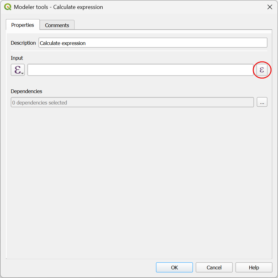
- We will use the expression function
layer_property()to get a count of features for the input layer. Enter the expression as shown below and click OK..
layer_property(@input_vector_layer, 'feature_count')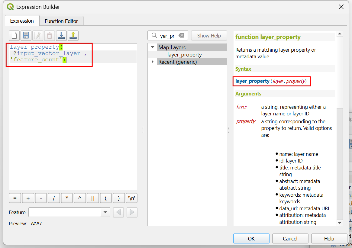
- Next locate the Modeler tools → Raise exception algorithm and drag it to the canvas.
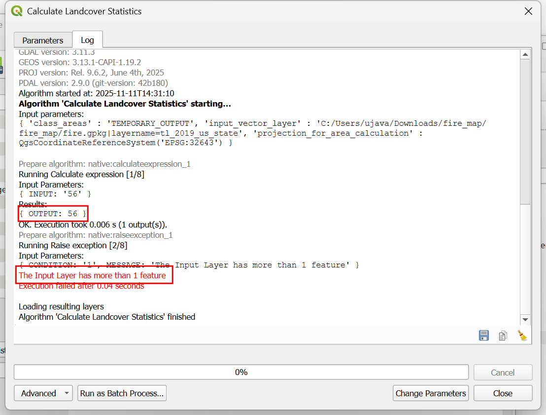
- In the **Modeler tools - Raise exception* dialog, enter
The Input Layer has more than 1 featureas the Error message. For the Condition, switch to Pre-calculated Value, enter the following expression. This configuration will throw an error when the number of features is greater than 1.
@Calculate_expression_OUTPUT > 1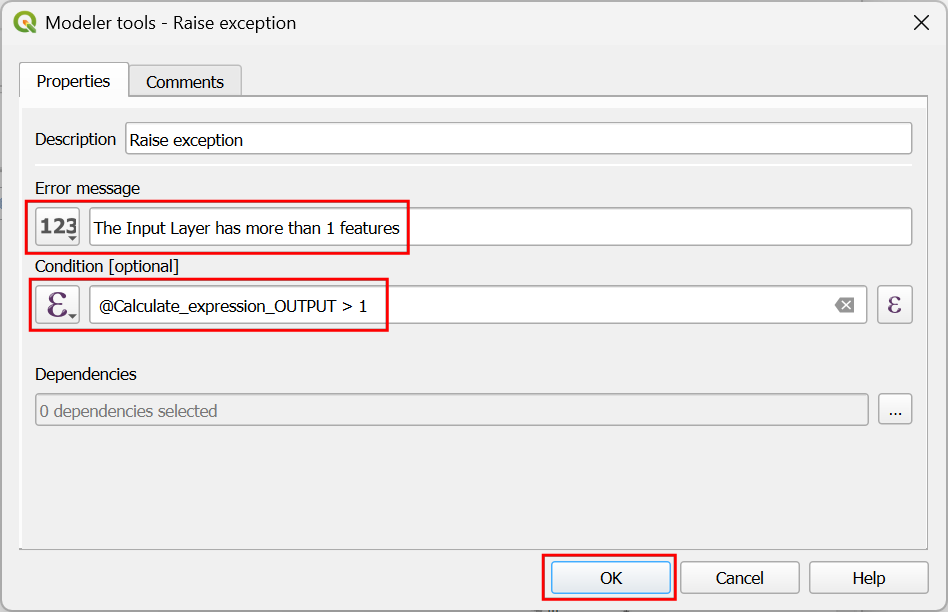
- We want the input validation to happen before any of the processing steps. So we add the validation as a dependency to the first step of the workflow. Click the box for Reproject layer.
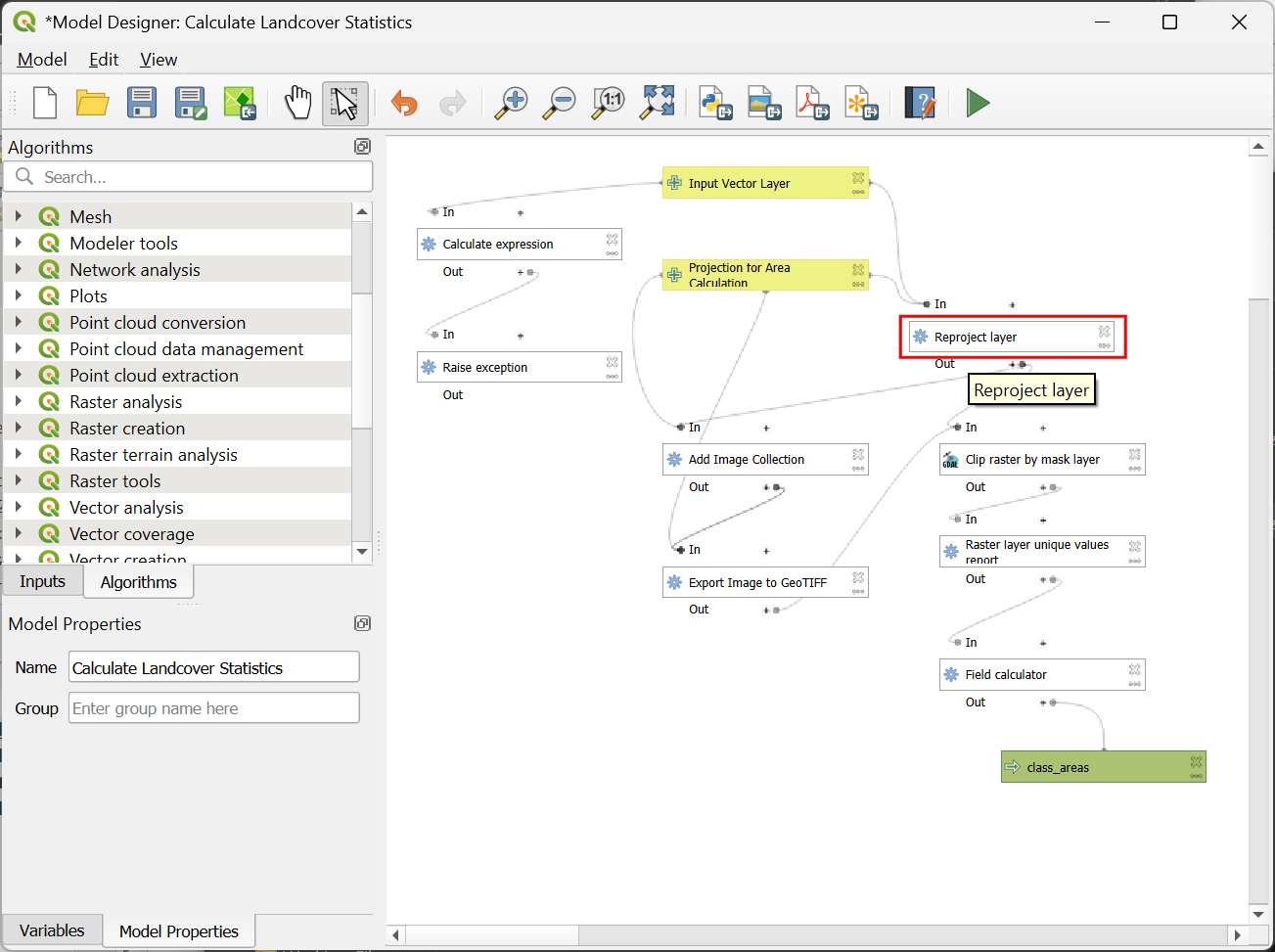
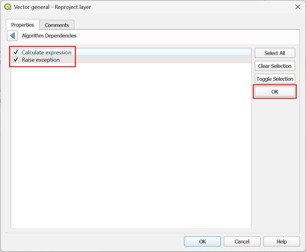
- In the Vector general - Reproject layer dialog, scroll down to the bottom and click the … button for Dependencies.
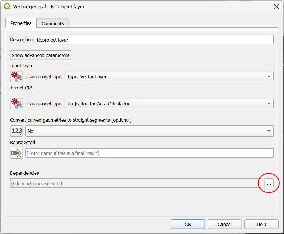
- Select both
Calculate expressionandRaise exceptionalgorithms and click OK. This will ensure these algorithms are completed before this step.
- Test the model by selecting any data layer having more than 1 polygon and you will see the exception raise by the model.
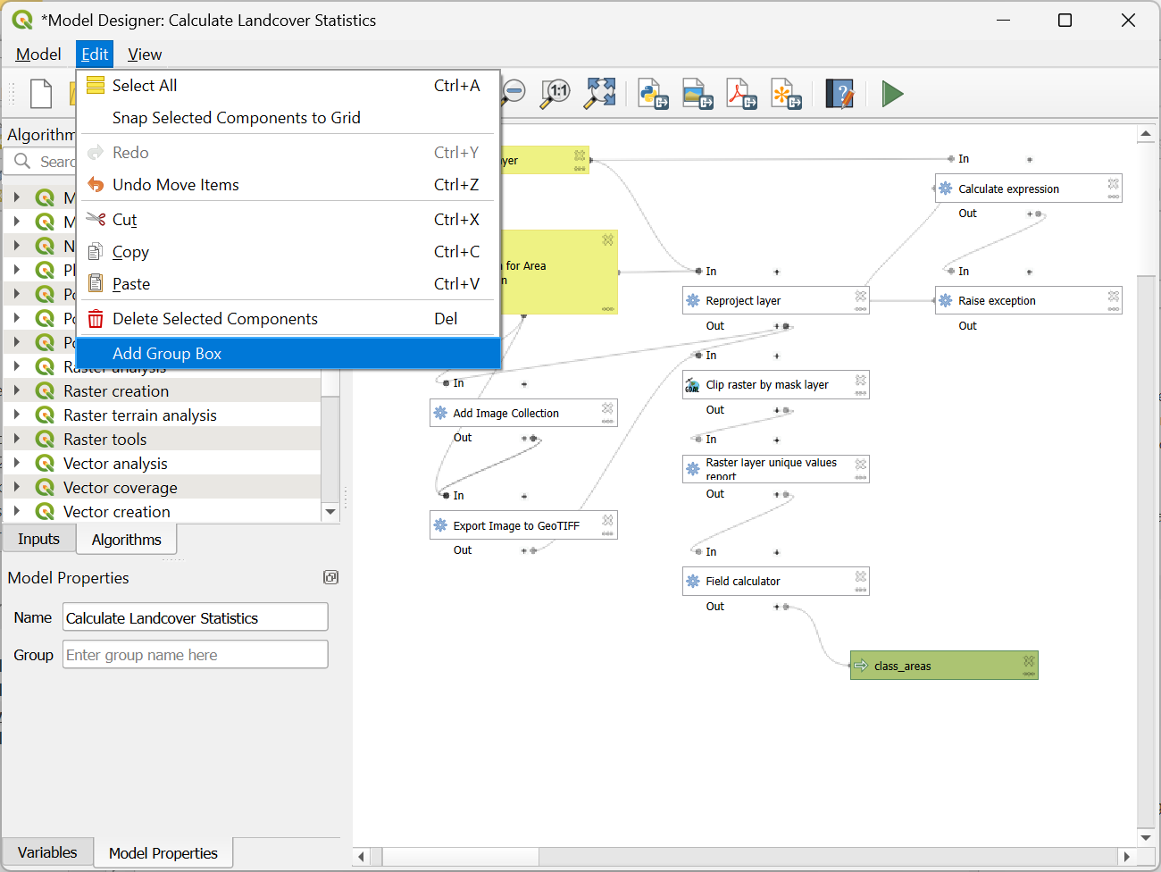
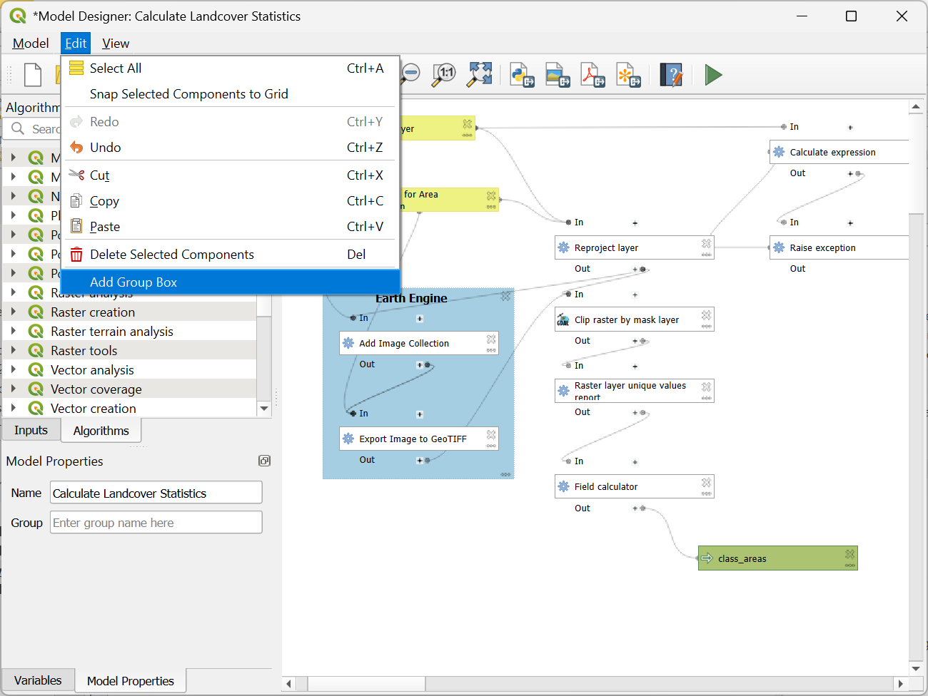
- It is a good practice to add some documentation to the model and add visual cues to help maintainers understand the workflow better. Let’s add a group box to group and label certain steps of the workflow. Go to Edit → Add Group Box.
- Click on the canvas to add a group box. Align it over the steps
related to Google Earth Engine. Double-click the box and enter the
Title as
Earth Engineand select a color of your choice.
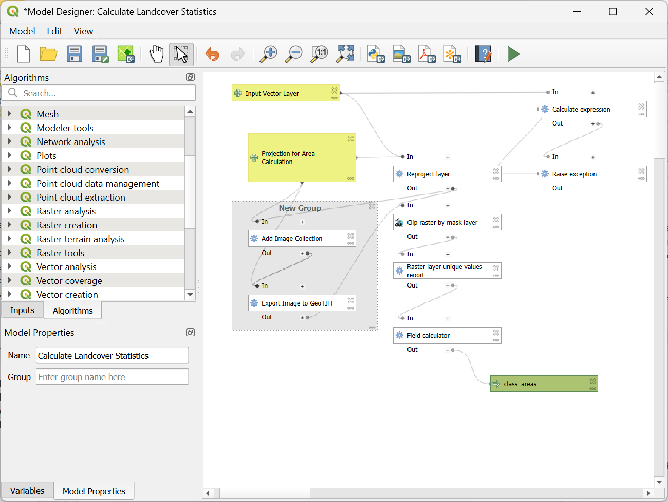
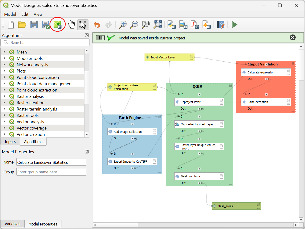
- Similarly add group boxes for the steps related to QGIS processing and input validation.
- Now the model is complete. Save it in the QGIS project.
If you’d like to catch up to this point, you can load the
Model_Designer_Checkpoint2.qgz file in the
solutions folder of the data package.
Data Credits
- Sentinel-2 Level-2A: Contains Copernicus Sentinel data.
- Zanaga, D., Van De Kerchove, R., Daems, D., De Keersmaecker, W., Brockmann, C., Kirches, G., Wevers, J., Cartus, O., Santoro, M., Fritz, S., Lesiv, M., Herold, M., Tsendbazar, N.E., Xu, P., Ramoino, F., Arino, O., 2022. ESA WorldCover 10 m 2021 v200. (doi:10.5281/zenodo.7254221)
License
This workshop material is licensed under a Creative Commons Attribution 4.0 International (CC BY 4.0). You are free to re-use and adapt the material but are required to give appropriate credit to the original author as below:
Cloud-based Remote Sensing with QGIS and Google Earth Engine by Ujaval Gandhi www.spatialthoughts.com
© 2025 Spatial Thoughts www.spatialthoughts.com
If you want to report any issues with this page, please comment below.